H100 CUDA Kernels for Gated Delta Net
Link to github respository: https://github.com/kingsleykimm/h100_gdn_cuda.
Gated Delta Net
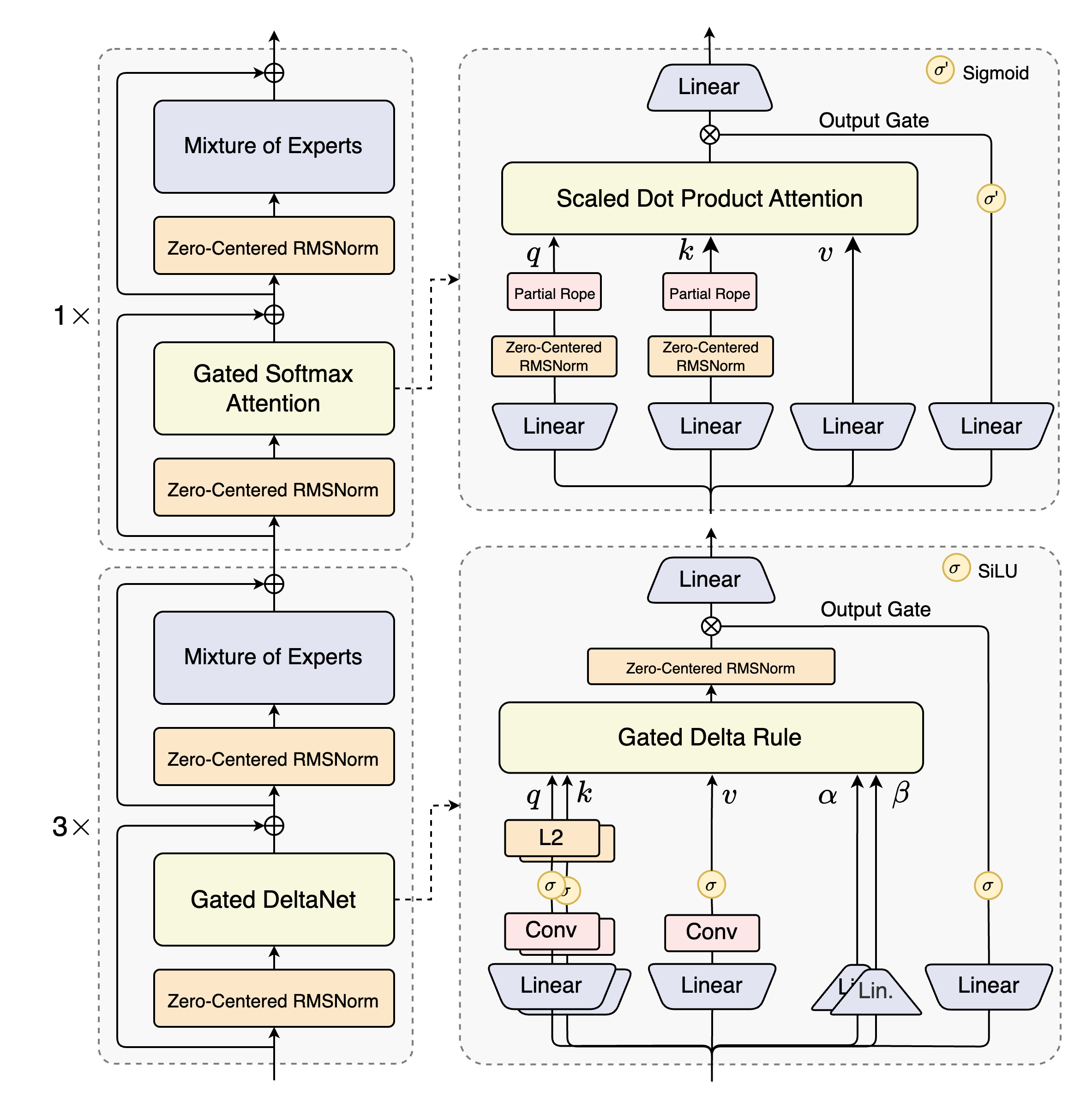
This section is part of my writing log for building a fully CUDA/CuTLASS inference engine for the Qwen3-Next-Thinking-FP8 model. We're looking specifically at the Gated Delta Net portion of a single layer, the Gated Delta Rule block in this image:
After writing it as part of my custom CUDA inference engine, I decided in light of iteration speed I would branch it off into a different package, the github repository is linked. Feel free to clone the repository and play around with the kernels - I'll mention some future optimizations I would like to do at the end of the post.
Gated Deltanet was first introduced by NVIDIA/MIT researchers in their paper, and Songlin Yang's (first author) accompanying blog post is a great learning resource as well, which I will reference frequently. It can be thought of as unifying two previously successful linear attention models: Mamba2 and vanilla DeltaNet, by taking the data-dependent gate decay term from Mamba2 and the delta rule from DeltaNet, which also has connections to Test Time Training and gradient descent on associative recall.
Why GDN? Why Qwen3-Next?
Qwen3-Next is the Qwen team's first push into exploring hybrid attention models, which have increasingly become popular due to their reduced memory requirements. As seen in the layer block, hybrid attention models contain both a mixture of normal attention blocks and linear attention blocks.
Linear Attention modifies the original attention formula by removing the softmax on the attention score matrix, which allows the attention operation to be linear. Linearity allows researchers to tap into the vast library of linear algebra tricks, creating more computationally efficient kernels, reaching subquadratic complexity. Hybrid attention models also win on memory -- instead of storing a $O(N)$ sized KV-cache per layer, we instead store a constant sized state matrix per layer.
I thought GDN was an interesting challenge to take on - it's popular but also orthogonal from the common QKV attention kernels that have been optimized over and over again. Custom linear attention architectures are only going to get more popular from now on, so it didn't hurt that I was building a popular variant completely from scratch. I also think it served as a unique challenge compared to implementing other production attention kernels like Flash-Decode because of the limited implementations online. I believe that there isn't a single CUDA + CuTLASS open source implementation, only Triton. (Although it looks like llama.cpp implemented a Qwen3-Next GDN implementation, but only through the ggml library and not through CUDA alone)
This meant there was no "follow-along" tutorial in the form of open-source code. I had to write the CUDA from scratch . The first challenge was translating the Triton implementations into CUDA - I used FLA's Triton kernels for inspiration. It forced me to think first in the perspective of the Triton authors, and understand the intent behind their kernel structure, and how they handled some interesting issues with recurrence and dependence between inputs and outputs. More on that in later sections.
Another great source just for learning SM90 optimizations and better TMA/GEMM tricks is the DeepGEMM library - I actually wrote a couple posts about their fp8 GEMMs and what I found fun about them. Reading their code helped me to grasp persistent CTA scheduling, and how to best overlap GEMMs using PTX+CUDA. More on that later as well.
All in all this was a fun project - definitely the technically hardest portion of the Qwen3-Next forward pass. I think I began brainstorming my plan of attack on 12/22/25, and verified the first forward pass (with nice shapes) about a month later. I hope this write up serves to give some insight into some SM90 optimization tricks as well as my thought process.
Notation
I'm going to copy over the notation and linear equation equations from the blog, which will be helpful to keep track of chunks.
Denoting $\mathbf{S}_{[i]} := \mathbf{S}_{iC} \in \mathbb{R}^{d \times d}, \square_{[i]} = \square_{iC+1:(i+1)C} \in \mathbb{R}^{C \times d}$ for $\square \in {\mathbf{Q}, \mathbf{K}, \mathbf{V}, \mathbf{O}}$. $\square_{[i]}^r = \square_{iC + r}$ for $\square \in {\mathbf{q}, \mathbf{k}, \mathbf{v}, \mathbf{o}, \mathbf{S}}$ and $r \in [0, C-1]$.
Using this notation, I can write the normal linear attention update:
$$ \mathbf{S}^r_{[i]} = \mathbf{S}_{[i]} + \sum_{t=1}^{r} \mathbf{v}^t_{[i]} \mathbf{k}^{t \top}_{[i]} $$
$$ \mathbf{o}^r_{[i]} = \mathbf{S}^r_{[i]} \mathbf{q}^r_{[i]} = \mathbf{S}_{[i]} \mathbf{q}^r_{[i]} + \sum_{t=1}^{r} \mathbf{v}^t_{[i]} (\mathbf{k}^{t \top}_{[i]} \mathbf{q}^r_{[i]}) $$
and in matrix form,
$$ \mathbf{S}_{[t+1]} = \mathbf{S}_{[t]} + \mathbf{V}^{\top}_{[t]} \mathbf{K}_{[t]} \in \mathbb{R}^{d \times d} $$
$$ \mathbf{O}_{[t]} = \mathbf{Q}_{[t]} \mathbf{S}^{\top}_{[t]} + (\mathbf{Q}_{[t]} \mathbf{K}^{\top}_{[t]} \odot \mathbf{M}) \mathbf{V}_{[t]} \in \mathbb{R}^{C \times d}$$
The matrix form conversion comes is because the sum of outer products is equivalent to a matrix multiplication (Tensor Cores!). $$ \sum_{i=1}^t a_i b_i^T = A_t B_t^T \newline A_t = \begin{bmatrix} a_1 & a_2 & \cdots & a_t \end{bmatrix} \newline B_t = \begin{bmatrix} b_1 & b_2 & \cdots & b_t \end{bmatrix} $$
Notice I get some more discounts in memory - in the matrix form equations the state updates are done over chunks of size $C$, so I only need to store state at intervals of $C$, giving us an effective memory savings of $1/C$.
Forward Pass
I really think reading both Part 1 and Part 2 of Songlin Yang's blog are prerequisites for this section. I also don't want to focus too heavily on the mathematical tricks and background of linear attention. The blog and paper do a much better job than I could do. Instead, I want to only focus on the key equations (the GDN recurrent rule) and how it is reforumlated for the chunkwise parallel pass. Notice that I will only be focusing on the chunked pass, which is when the number of total input tokens exceeds 32, so I can use Tensor Core MMAs, but the github also contains a recurrent implementation. I'll still copy over the equations and give some explanations.
Let's first take a look at the entire forward pass defined in FLA. The general idea is that we take three input tensors, $\mathbf{Q}, \mathbf{K}, \mathbf{V}$ similar to vanilla attention, but we also take some extra gating terms, the $g_t, \beta_t$ tensors that weight how much we want to remember previous context and how much we want to overwrite current memory, respectively.
This is the core of GDN, and the Mamba2 architecture it builds on - we maintain a persistent state, similar to RNNs that lives separately from the QKV tensors. Vanilla attention has an implicit state through the massive $\text{softmax}\left ( \mathbf{QK^T} \right)$ matrix it calculates every forward pass.
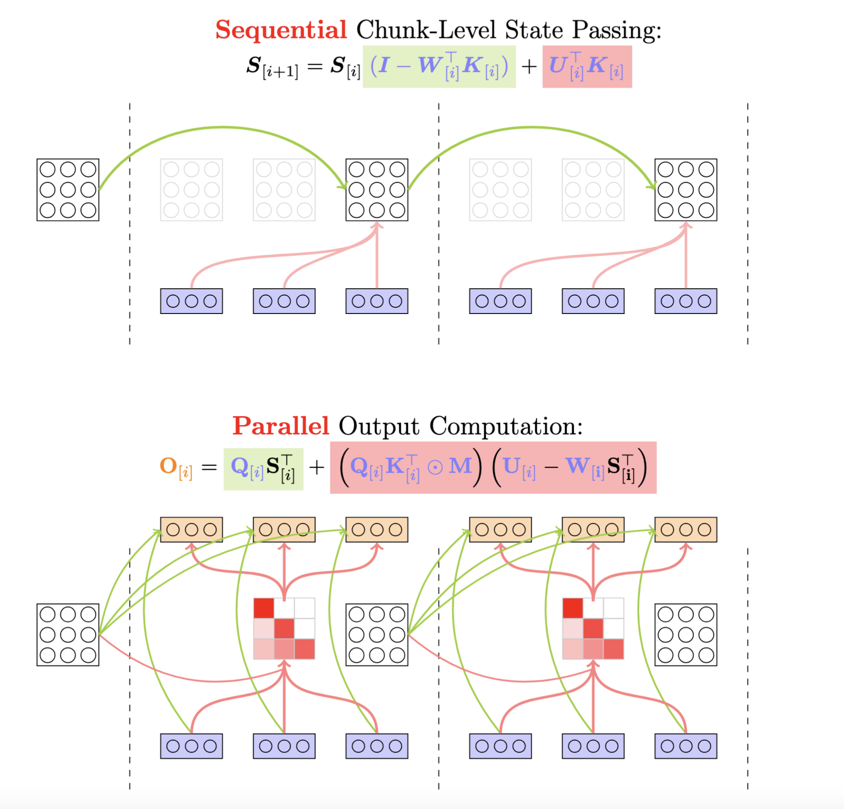
I'm going to paste in an image from Songlin Yang's blog that provides some visual intuiton for the forward pass, and we'll break down the differenet equations in chapters throughout this post.
You'll notice that the $\mathbf{U}, \mathbf{W}$ matrices weren't included as inputs in the GDN block - these are intermediary matrices that need to be calculated to convert the recurrent nature of the gated delta rule into a chunkwise parallel form, reflecting the concept of state space duality (SSD) from Mamba2. The next section has more information on this.
UW Computation
The U and W matrices are an essential part of the forward pass - to understand their role I need to first look at the unrolled recurrent equation, and then dip into graph theory. Again, the GDN blog is a much better resource on this. What I'll do is paste in some of their equations and explain what each does.
I start with the recurrent delta net update rule.
Delta Net's Recurrent Update Rule
Delta Net combines the linear attention update with the delta rule. The delta rule is a simple first-order recurrence taht adjusts parameters based on a delta, calculated as the difference between the target value and the current prediction.
$$ \mathbf{S}_t \in \mathbb{R}^{\mathbf{d_v} \times \mathbf{d_k}},\quad \mathbf{k}_t \in \mathbb{R}^{\mathbf{d_k}},\quad \mathbf{v}_t \in \mathbb{R}^{\mathbf{d_v}} \newline \mathbf{S}_t = \mathbf{S}_{t-1} - \beta_t \left(\mathbf{S}_{t-1} \mathbf{k}_t - \mathbf{v}_t\right)\mathbf{k}_t^T \newline = \mathbf{S}_{t-1}(I - \beta_t \mathbf{k}_t \mathbf{k}_t^T) + \beta_t \mathbf{v}_t \mathbf{k}_t^T $$
In the gated variant, we also add the gating term $g_t$.
Gated Delta Net version:
$$
\mathbf{S}_t = \mathbf{S}_{t-1}(g_t(I - \beta_t \mathbf{k}_t \mathbf{k}_t^T)) +\beta_t \mathbf{v}_t \mathbf{k}_t^T
$$
The $g_t$ value is the data-dependent gating term, which is used to control the state decay. The $\beta_t$ value is the data dependent writing strength, and the $S_{t-1}$ value is the previous state, and the $k_t$ value is the current key, and the $v_t$ value is the current value. This new form of the gated delta rule shows that we have a transition matrix: $g_t(I - \beta_t \mathbf{k}_t \mathbf{k}_t^T)$, and an update term: $\beta_t \mathbf{v}_t \mathbf{k}_t^T$.
Naturally, we don't want to directly compute this recurrent update step by step on very large sequence lengths and ideally we find a representation that uses only matrix operations. Let's unroll the recurrence (for delta net):
$$ \mathbf{S}_t = \mathbf{S}_{t-1} (I - \beta_t \mathbf{k}_t \mathbf{k}_t^T) + \beta_t \mathbf{v}_t \mathbf{k}_t^T \newline = \sum_{i=1}^t \beta_i (\mathbf{v}_i \mathbf{k}_i^T) \left ( \prod_{j=i+1}^t (I - \beta_j \mathbf{k}_j \mathbf{k}_j^T) \right) $$
Like the linear attention above, we chunk the $t$ term (sequence length) into chunks of size $C$, so our unrolled recurrence gets split up more. Note here that we're going to use the chunk notation:
$$ \mathbf{S}^{r}_{[i]} = \mathbf{S}_{[i]} \prod_{t=1}^{r} \left( \mathbf{I} - \beta^{t}_{[i]} \mathbf{k}^{t}_{[i]} (\mathbf{k}^{t}_{[i]})^{\top} \right) + \sum_{t=1}^{r} \left( \beta^{t}_{[i]} \mathbf{v}^{t}_{[i]} (\mathbf{k}^{t}_{[i]})^{\top} \prod_{s=t+1}^{r} \left( \mathbf{I} - \beta^{s}_{[i]} \mathbf{k}^{s}_{[i]} (\mathbf{k}^{s}_{[i]})^{\top} \right) \right) $$
All we did is include some more indices. The second term represents the intra-chunk state at timestep $r$, which we add to the first step, the cumulative productive of transition matrices, beginning from our start state for the current chunk. However, we also need the first step inside a chunk to include information from previous chunks, otherwise causality is broken. Later, we'll see how the chunks are computed sequentially to accumulate information.
However, this formulation still contains too many cumulative products and sums. We fix this by introducing the WY representation of Householder matrices.
WY Representation
The transition matrix $(I - \beta_t k_t k_t^T)$, when $\beta_t = 2$ is a Householder Matrix, a special group of matrices. A paper (linked in the blog) introduces the WY representation, which allows the cumulative products of Householder matrices to be written as a sum of outer products:
$$
Q_k = \mathbf{P}_1 \mathbf{P}_2 \cdots \mathbf{P}_k, \hspace{1cm} \mathbf{P}_i \in \mathbb{R}^{d \times d} \newline
Q_k = \mathbf{I} + \mathbf{W}\mathbf{Y}^T, \hspace{1cm} \mathbf{W} \in \mathbb{R}^{d \times k}, \mathbf{Y} \in \mathbb{R}^{k \times d}
$$
The GDN blog and paper extend this result to the state matrix and the transition matrix: $$ \prod_{i=1}^t (\mathbf{I} - \beta_i \mathbf{k}_i \mathbf{k}_i^T) = \mathbf{I} - \sum_{i=1}^t \mathbf{w}_i \mathbf{k}_i^T \newline \mathbf{S}_t = \mathbf{S}_{t-1}(\mathbf{I} - \beta_t \mathbf{k}_t \mathbf{k}_t^T) + \beta_t \mathbf{v}_t \mathbf{k}_t^T = \sum_{t=1}^n \mathbf{u}_t \mathbf{k}_t^T \tag{1} $$
See the blog / paper for the inductive proofs.
Substituting these equations back into the chunkwise gated delta rule gives: $$ \mathbf{S}^{r}_{[i]} = \mathbf{S}_{[i]} \left( \mathbf{I} - \sum_{t=1}^{r} \mathbf{w}_{[i]}^t \mathbf{k}_{[i]}^t \right) + \sum_{t=1}^{r} \mathbf{u}_{[i]}^t \mathbf{k}_{[i]}^t $$
Currently, both vectors have a recursive formulation: $$ \mathbf{w}^{r}_{[t]} = \beta^{r}_{[t]} \left( \mathbf{k}^{r}_{[t]} - \sum_{i=1}^{r-1} \mathbf{w}^{i}_{[t]} (\mathbf{k}^{i}_{[t]})^{\top} \mathbf{k}^{r}_{[t]} \right) \tag{2} $$ $$ \mathbf{u}^{r}_{[t]} = \beta^{r}_{[t]} \left( \mathbf{v}^{r}_{[t]} - \sum_{i=1}^{r-1} \mathbf{u}^{i}_{[t]} (\mathbf{k}^{i}_{[t]})^{\top} \mathbf{k}^{r}_{[t]} \right) \tag{3} $$ This is computable using a CUDA kernel - the obvious issue is how inefficient the kernel would be, because it computes a single vector at a time, needs to reaccess all previous vectors. With how large prefill token counts are, this would not be feasible. The $\mathbf{w}$ and $\mathbf{u}$ vectors are also computed starting from the first position in each chunk, which hints at some sort of parallelism across chunks.
The GDN paper provides a method of reformulating the recursive equations into matmuls, using graph theory.
Graph Theory
Let's say we have a graph where each node represents a sequence position, so each node is $w_i \forall i \in [1, n]$. For the current update, the cumulative sum is only up to $i = n-1$. This hints at a causal dependency between nodes, which allows us to define a weighted Directed Acyclic Graph (DAG).
What are the weights here? What happens if we set each edge weight to $-\beta_t \mathbf{k_i^Tk_n}$?
Then the sum of the weights of all paths from node $j$ to node $i$ is exactly the second term in the equation, $-\beta_n \sum_{t=1}^{n-1} (w_t(\mathbf{k_t^Tk_n}))$. And since this is a weighted DAG, graph theory tells us how to compute this efficiencly using the inverse of the adjacency matrix, here's an excerpt from the blog:
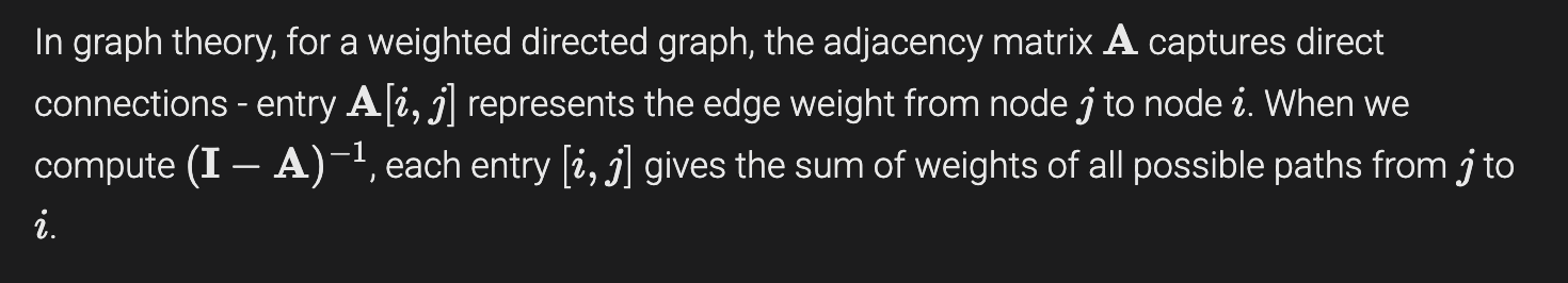
Again, the $\mathbf{w_n}, \mathbf{u_n}$ recursions are the exact same format, so they have the same adjacency matrix, the only difference is the nodes, so we can look at one of them and find the equations for other as well. We can now define this adjancency matrix, since we know how the weights are structured: $$ \text{Let: }K_t \in \mathbb{R}^{n \times d_k}, \text{where n is sequence length} \newline A_t = \text{tril} (-\text{diag} (\beta_t) K_t K_t^T, -1), A_t \in \mathbb{R}^{n \times n} $$ Notice the lower triangular operator to enforce the causal dependency. Because $A_t$ is lower triangular, $T_t = (I - A_t)^{-1}$ will be lower triangular with ones on the diagonal, which allows us to use forward substitution to compute the inverse. This takes an originally $O(n^3)$ operation and reduces it to $O(n^2)$. Now, each $T_t [i, j]$ is the sum of the weights of all paths from node $j$ to node $i$.
In order to combine the first and second terms in the equation, we perform the matmul: $T_t \text{diag}(\beta_t) K_t$.
$T_t \text{diag}(\beta_t)$ is lower triangular, with $\beta_t$ on the diagonals. The matmul can be interpreted as each row of $T_t$ performing a linear combination on the key vectors where $i < j$, and then multiplying the $k_j$ vector with the $\beta_t$ term. This is equivalent to the recursive update equations, which can be seen by unrolling the equations for a few steps.
So both the U and W now have efficient matmul implementations: $$ T_{[t]} \in \mathbb{R}^{n \times n}, K_{[t]} \in \mathbb{R}^{n \times d_k}, V_{[t]} \in \mathbb{R}^{n \times d_v}, \beta_{[t]} \in \mathbb{R}^n \newline W_{[t]} = T_{[t]} \text{diag}(\beta_{[t]}) K_{[t]}, \hspace{1cm} W_{[t]} \in \mathbb{R}^{n \times d_k} \newline U_{[t]} = T_{[t]} \text{diag}(\beta_{[t]}) V_{[t]}, \hspace{1cm} U_{[t]} \in \mathbb{R}^{n \times d_v} \tag{4} $$
UW Kernel
Here's the triton function signature for the UW kernel:
    g = chunk_local_cumsum(g, chunk_size=64, cu_seqlens=cu_seqlens)
    # obtain WY representation. u is actually the new v.
    A = chunk_scaled_dot_kkt_fwd(
        k=k,
        g=g,
        beta=beta,
        cu_seqlens=cu_seqlens,
        output_dtype=torch.float32,
    )
    A = solve_tril(
        A=A,
        cu_seqlens=cu_seqlens,
        output_dtype=k.dtype,
    )
    w, u = recompute_w_u_fwd(
        k=k,
        v=v,
        beta=beta,
        A=A,
        g=g,
        cu_seqlens=cu_seqlens,
    )
Here's my CUDA function signature:
template <uint32_t SHAPE_K, uint32_t SHAPE_V, uint32_t kBatchSize, uint32_t kChunkSize, uint32_t kNumVHeads,
          uint32_t kNumKHeads, uint32_t BLOCK_K, uint32_t kNumBlocks, uint32_t kNumTMAMulticast,
          uint32_t kNumTMAThreads, uint32_t kNumMathThreads, uint32_t kSwizzleKMode, uint32_t kSwizzleVMode,
          uint32_t kSwizzleAMode, uint32_t kSeqLen, bool kIsVarLen, uint32_t kUseGating>
__global__ void __launch_bounds__(kNumMathThreads + kNumTMAThreads, 1)
    sm90_bf16_compute_u_w(CUTE_GRID_CONSTANT const cute::TmaDescriptor k_tensor_map,
                          CUTE_GRID_CONSTANT const cute::TmaDescriptor v_tensor_map,
                          CUTE_GRID_CONSTANT const cute::TmaDescriptor u_tensor_map,
                          CUTE_GRID_CONSTANT const cute::TmaDescriptor w_tensor_map,
                          CUTE_GRID_CONSTANT const cute::TmaDescriptor beta_tensor_map,
                          CUTE_GRID_CONSTANT const cute::TmaDescriptor gate_tensor_map, int batch_size, int shape_T,
                          int chunk_indices_length, int *chunk_indices, int *cu_seqlens, __nv_bfloat16 *U_ptr,
                          __nv_bfloat16 *W_ptr, float *gate_ptr)
In the Triton implementation, the UW kernel splits into three separate kernels:
- chunk_scaled_dot_kkt_fwd: Computes the per-chunk adjacency matrix $A_t$
- solve_tril: Computes the inverse of $A_t$
- recompute_w_u_fwd: Computes the W and U matrices, parallelized across chunks
The chunk_local_cumsum kernel is a simple kernel that computes the cumulative sum of the gating term $g_t$ along the sequence length dimension, which allows us to directly multiply the gating terms instead of computing the cumsum inside the UW kernel. Kernels 1 and 3 are straightforward matmuls, which can be implemented with Tensor Cores. Kernel 2 implements forward substitution.
What I noticed was that the $KK^T$ kernel computes the adjacency matrix fully, but then stores it back into global memory. Then in the solve_tril kernel, I immediately load it back from global memory. Not to mention this is another kernel launch. I also know that the adjacency matrix isn't used in other parts of the forward pass - it is only needed to compute U and W and is chunk-local, so we don't need to worry about sychronization across SMs. So storing it back to global memory is unnecessary.
Let's just fuse these three kernels together then. We can compute the $\mathbf{KK^T}$ result, which is stored in registers on SM90's Tensor Cores, called Warpgroup MMAs, because a warpgroup of 128 threads coordinate to perform a matmul operation, and perform a RMEM to SMEM copy on the result using the PTX instruction stmatrix.sync (intended for WGMMA accumulator layouts). Then I can implement the forward substition on SMEM (without any global memory loads/stores), and compute the final matmul seen in Equation (1).
The compute_u_w kernel can be found here.
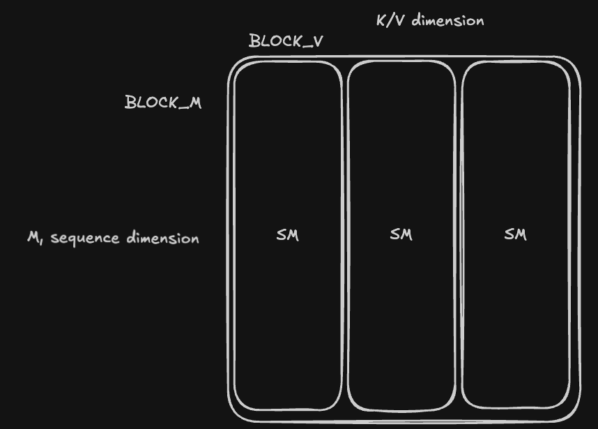
GDN Scheduler
The Persistent GDN scheduler was inspired by the Persistent DeepGEMM scheduler, which tiles the output matrices across the SM grid. There are two variants of the GDN scheduler - the ChunkGDNScheduler and RecurrentGDNScheduler.
The former is used in the chunkwise parallel kernels, while the latter is used for recurrent (sequential) kernels. Both are nearly the same, just some minor differences because the Recurrent form doesn't split along the sequence dimension -- each CTA will own an entire batch.
Here is the definition for the ChunkGDNScheduler
// ChunkGDNScheduler - Persistent scheduler for chunked GDN (Gated Delta Networks)
// Handles both varlen (packed sequences) and fixed padded settings
// BLOCK_M = chunk size (always 64)
// kNumHeads = number of query heads
// kNumSMs = number of blocks across the gridDim for persistent scheduling
// kIsVarLen = compile-time flag for varlen vs padded mode
template <uint32_t BLOCK_M, uint32_t kNumVHeads, uint32_t kNumKHeads, uint32_t kNumBlocks, uint32_t BLOCK_V,
          bool kIsVarLen = false>
struct ChunkGDNScheduler {

  // Runtime parameters
  int batch_size;
  int num_chunks;     // total number of chunks across all batches
  int *cu_seqlens;    // cumulative sequence lengths [batch_size + 1], only used in varlen mode
  int *chunk_indices; // shape (num_chunks, 2) linearized - pairs of [batch_idx, chunk_idx]
  int num_v_blocks;
  // For padded mode
  int max_seq_len;

  // Scheduler state
  int current_iter;
  int cur_block_idx;
  int num_blocks; // total blocks = num_chunks * kNumHeads

  int seq_start;
  int seq_end;
  int seq_len;

  // Varlen mode constructor
  __device__ __forceinline__ ChunkGDNScheduler(int batch_size, int shape_v, int num_chunks, int *cu_seqlens,
                                               int *chunk_indices)
      : batch_size(batch_size), num_chunks(num_chunks), cu_seqlens(cu_seqlens), chunk_indices(chunk_indices),
        num_v_blocks(ti_ceil_div(shape_v, BLOCK_V)), max_seq_len(0), current_iter(-1) {
    CUTE_STATIC_ASSERT(kIsVarLen, "Cannot use varlen constructor with padded mode");
    num_blocks = num_chunks * kNumVHeads * num_v_blocks;
  }

  // Padded mode constructor
  __device__ __forceinline__ ChunkGDNScheduler(int batch_size, int shape_v, int max_seq_len)
      : batch_size(batch_size), num_chunks(0), cu_seqlens(nullptr), chunk_indices(nullptr),
        num_v_blocks(ti_ceil_div(shape_v, BLOCK_V)), max_seq_len(max_seq_len) {
    CUTE_STATIC_ASSERT(!kIsVarLen, "Cannot use padded constructor with varlen mode");
    // For padded mode, calculate num_chunks from batch_size and max_seq_len
    int chunks_per_batch = ti_ceil_div(max_seq_len, (int)BLOCK_M);
    num_chunks = batch_size * chunks_per_batch;
    num_blocks = num_chunks * kNumVHeads * num_v_blocks;
    current_iter = -1;
  }
};
The kIsVarLen template parameters determines whether I are in VarLen (variable length) or padded mode. VarLen is a technique that packs all incoming tokens across batches across the sequence dimension, to avoid the use of padding tokens. It's important in prefill scenarios where the sequence lengths across a batch vary, and there is wasted computation on padding tokens. Padded mode is the familiar setting where each sequence in a batch is padded to the max sequence length in the batch.
The cu_seqlens and chunk_indices are varlen metadata, which are used to locate the sequence start to end indices that the SM calculates on each persistent iteration. More information can be seen in the get_next_block function, but here's a short code snippet showing their function:
int v_head_blocked_idx = cur_block_idx / kNumVHeads;
v_block_idx = v_head_blocked_idx % num_v_blocks;
head_idx = cur_block_idx % kNumVHeads;
int global_chunk_idx = v_head_blocked_idx / num_v_blocks;
if constexpr (kIsVarLen) {
    // Load batch_idx and chunk_idx from precomputed chunk_indices
    // chunk_indices is linearized as [batch_idx_0, chunk_idx_0, batch_idx_1, chunk_idx_1, ...]
    int2 indices = __ldg(reinterpret_cast<int2 *>(chunk_indices + global_chunk_idx * 2));
    batch_idx = indices.x;
    chunk_idx = indices.y;

    // Compute sequence boundary for masking in varlen mode
    // Get sequence length for this batch
    int global_seq_start = __ldg(cu_seqlens + batch_idx);
    int global_seq_end = __ldg(cu_seqlens + batch_idx + 1);

    seq_start = global_seq_start + chunk_idx * BLOCK_M;
    seq_end = seq_start + BLOCK_M;
    // Check if sequence ends within this chunk
    if (seq_end > global_seq_end) {
    // seq_end_in_chunk is the last valid row index (0-indexed within chunk)
    seq_end_in_chunk = BLOCK_M - 1 - (seq_end - global_seq_end);
    seq_len = seq_end_in_chunk + 1;
    } else {
    seq_end_in_chunk = -1; // no boundary in this chunk, or chunk is fully valid
    seq_len = BLOCK_M;
    }
}
This code snippet is from the get_next_block function in the Scheduler class. The chunk indices array, like the comments says is (num_sequences, 2) sized array with pairs of (batch_idx, chunk_idx) for each chunk. global_chunk_idx, which is the chunk index the current CTA is assigned to, loads the batch_idx and chunk_idx for the current CTA.
Using the batch_idx, we can load the sequence start and end indices from the cu_seqlens array, which is a cumulative sum of the sequence lengths for each batch, giving us the boundaries for masking in the later TMA stores. We define a few more scheduler variables for boundary metadata: seq_start, seq_end, seq_end_in_chunk.
seq_start is also used to locate the global row we should offset for the TMA loads and stores. seq_end_in_chunk represents the last valid row index within the chunk, so on ragged chunks, I used a manual unrolled loop to store only valid rows by checking with this variable (see TMA Store section for more details). You'll notice that all this extra work can be succintly defined in Triton by using block masking, but we're going with manual CUDA here.
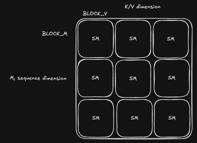
The other parameters are all problem shape parameters. The M dimension is always the sequence dimension, ($n$ in Equation (1)). BLOCK_M is the chunk size over the sequence dimension - I actually hardcode this to 64 to align with the atomic unit of WGMMAs, where M is always 64. BLOCK_V is the chunk size over the value dimension, ($d_v$ in Equation (1)). For the kernels, I actually assume that $d_k = d_v$ for now, it looks like most of the models integrating GDN make this assumption as well. So BLOCK_V is also BLOCK_K for the key dimension.
Then both the U and W matrices follow this tiling:
Main Kernel Body
The bodies for all kernel follow the same structure:
- First load in all the metadata, like warp and lane indices, smem offsets, tensor maps
- Set up shared memory pointers and barrier initialization
- Set up WGMMA selectors to find the correct WGMMA CuTe types.
- Using warpgroup specialization, split into either TMA or Math warpgroups.
In the TMA warpgroup, I issue the first wave of stores:
/*
global_row_offset is the sequence index offset for the current chunk, calculated by the scheduler.
*/

auto &barrier = tma_barrier[0];
for (int k_block_idx = 0; k_block_idx < num_k_blocks; k_block_idx++) {
    tma_copy<BLOCK_K, kChunkSize, kSwizzleKMode, __nv_bfloat16, 3>(
        &k_tensor_map, &barrier, sK + k_block_idx * BLOCK_K * kChunkSize, k_block_idx * BLOCK_K, k_head_idx, 1,
        global_row_offset);
}
// Load all V blocks
tma_copy<SHAPE_V, kChunkSize, kSwizzleVMode, __nv_bfloat16, 3>(&v_tensor_map, &barrier, sV, 0, head_idx, 1,
                                                                global_row_offset);
The tma_copy function has the signature
template <int BLOCK_INNER, int BLOCK_OUTER, size_t SWIZZLE_SIZE, typename tdtype_t, int NDIM = 2>
__device__ __forceinline__ void tma_copy(void const *tensor_map, cutlass::arch::ClusterTransactionBarrier *barrier,
                                         tdtype_t *smem_addr, uint32_t inner_idx, uint32_t outer_idx, int num_multicast,
                                         uint32_t crd2_idx = 0, uint32_t crd3_idx = 0, uint32_t crd4_idx = 0)
It is a router function that selects one of cute's SM90_(NDIM)D_TMA_COPY methods, based on the NDIM provided, and if num_multicast is greater than 1, I use the multicast version. For the current UW kernel, I only need to load in the $\mathbf{K_{[t]}}$ and $\mathbf{V_{[t]}}$ tensors. I also omitted some if cases between the padded and varlen mode for brevity, but please check the code for all the details.
The $\beta_t$ tensor, and optionally the $g_t$ tensor for Gated Delta Net are loaded later, in the Math warpgroups, since the vectors are only $C$ elements long, and don't need larger TMA loads.
bool can_load_gate_and_beta;
    uint32_t offset;
    if constexpr (kIsVarLen) {
    can_load_gate_and_beta = threadIdx.x < kChunkSize && (seq_end_in_chunk < 0 || threadIdx.x <= seq_end_in_chunk);
    offset = head_idx * beta_stride + global_row_offset;

    } else {
    can_load_gate_and_beta = threadIdx.x < kChunkSize && chunk_idx * kChunkSize + threadIdx.x < shape_T;
    offset = batch_idx * (kNumVHeads * beta_stride) + head_idx * beta_stride + chunk_idx * kChunkSize;
    }

    if (threadIdx.x < kChunkSize) {
        if (can_load_gate_and_beta) {
            if constexpr (kUseGating) {
            s_gate[threadIdx.x] = __ldg(gate_ptr + offset + threadIdx.x);
            }
            sBeta[threadIdx.x] = __ldg(beta_ptr + offset + threadIdx.x);
        } else {
            if constexpr (kUseGating) {
            s_gate[threadIdx.x] = 0.0f;
            }
            sBeta[threadIdx.x] = 0.0f;
        }
    }
Again, there a small split in the indexing logic between Varlen and Padded, since we use seq_end_in_chunk in the Varlen case to determine boundaries, instead of shape_T, which is the padded sequence length across all batches. The global_row_offset variable that keeps showing up is calculated as such:
int global_row_offset;
if constexpr (kIsVarLen) {
    global_row_offset = scheduler.seq_start;
} else {
    global_row_offset = batch_idx * kSeqLen + chunk_idx * kChunkSize;
}
Notice I just use the result already computed in the scheduler for Varlen, while for Padded, the shapes are well-defined and straightforward to compute. So the tensors we're working with (locally in each CTA) have these shapes: $\mathbf{K_{[t]}} \in \mathbb{R}^{C \times b_k}, \mathbf{V_{[t]}} \in \mathbb{R}^{C \times d_v}, \beta_t \in \mathbb{R}^C, g_t \in \mathbb{R}^C$.
In the Math warpgroup, we wait for the TMA stores to arrive, and then begin the first matmul. If you noticed in the TMA loads, we actually wanted $\mathbf{K_{[t]}}$ to be tiled across the $d_k$ dimension, since it'll be easier to compute $\mathbf{K_{[t]}} \mathbf{K_{[t]}}^T$.
Short sidenote on accumulator ($D$) layouts in SM90 WGMMA:
The accumulator layout for BF16 Tensor Core matmuls can be seen here. I followed DeepGEMM's code here to wrap the PTX wgmma instruction that takes in the Shared Memory Matrix Descriptors for A and B, as well a register array of shape $2 \times 2 \times N$ for the number of values each thread holds in $D$. Refer to the to see this matches.
Once the matmul completes, we perform postprocessing, like gating and storing from RMEM to SMEM.
#pragma unroll
for (int i = 0; i < KKTMMA::kNumAccum; i++) {
    auto [row, col] = get_accum_row_col(threadIdx.x, i);
    if (row != col) {
        accum[i] *=
            expf(s_gate[row] -
                s_gate[col]); // gets the cumulative gate product, by subtracting the row gate from the column gate
    }
}

#pragma unroll
for (int i = 0; i < KKTMMA::kNumAccum / 4; i++) {
    // zero-swizzle
    uint8_t *smem_ptr = reinterpret_cast<uint8_t *>(sA + a_row_index * kChunkSize + i * 8);
    // Each iteration stores 4 consecutive fp32 accumulators as 4 bf16 values
    // Scalar stores in row-major layout: sA[row * kChunkSize + col]
    custom_SM90_U32x2_STSM_N<__nv_bfloat162>::copy(__float22bfloat162_rn({accum[i * 4 + 0], accum[i * 4 + 1]}),
                                                    __float22bfloat162_rn({accum[i * 4 + 2], accum[i * 4 + 3]}),
                                                    smem_ptr);
}
cutlass::arch::NamedBarrier::sync(kNumMathThreads, 1); // ensure STSM writes are visible
The first part is only for gating scenarios -- it uses a smaller helper function to map the $(T,V) \to (r,c)$ in the output matrix, and then applies a position dependent gate decay term. The second loop is a standard SM90 STSM store
Why is the gate decay needed here though? Shouldn't it only be used in the state updates?
The Gate Decay Term
But remember how the $\mathbf{u_t}$ and $\mathbf{w_t}$ vectors are computed? They were computed recursively from the chunk-local state updates, which inherently include the gate decay term. The math gets a little too long for this post, but the proofs for the extended WY represenation for GDN can be found in Section 3.3 and Appendix A of their paper.
I'm going to also include the central GDN equations from the paper for reference, since this will help explain why and where I include the gate decay terms for each matrix. We'll reference this image later as well.
Only focus on the $\mathbf{U}_{[t]}, \mathbf{W}_{[t]}, \mathbf{u}_t, \mathbf{w}_t$ terms, and how they depend on the gate decay terms ($\gamma_t$) for now.
There is one slight error with the last $\mathbf{O_{[t]}}$ equation - with the gate decay the causal mask $\mathbf{M}$ should have the casual gating terms applied to it, which was shown earlier in the paper in the Mamba2 preliminaries:
The paper also explains the notation behind the different arrows above matrices, which represent the direction of decay that matches the recurrent rule. Unrolling the recurrent rules and tracing out the different gating terms and how they accumulate on each vector/matrix is a good exercise to understand the math and get some better intuition of the previously mentioned state space duality (SSD).
The final result from their proof shows modified state and $\mathbf{u_t, w_t}$ equations (the first two results are from the paper, the last $\mathbf{w}_t$ equation is straightforward by extending the blog's proof):
$$ \mathbf{S}_t = \sum_{i=1}^{t} \frac{\gamma_t}{\gamma_i} \mathbf{u}_i \mathbf{k}_i^{\top}, \qquad \mathbf{u}_t = \beta_t \left( \mathbf{v}_t - \sum_{i=1}^{t-1} \frac{\gamma_t}{\gamma_i} \mathbf{u}_i \mathbf{k}_i^{\top} \mathbf{k}_t \right) \qquad \mathbf{w}_t = \beta_t \left( \mathbf{k}_t - \sum_{i=1}^{t-1} \frac{\gamma_t}{\gamma_i} \mathbf{w}_i \mathbf{k}_i^{\top} \mathbf{k}_t \right) $$
Ok, so now the weights in the DAG I constructed earlier have a new form: $-\frac{\gamma_t}{\gamma_i} \beta_t \mathbf{k}_i^{\top} \mathbf{k}_t$. This is why I apply the specific gate decay term for each $\mathbf{A}_{[t]}[i, j ]$ entry. The reason it's not a division is because GDN is actually trained with the gate tensors stored in log space for numerical stability, which is why I multiply by $\exp(\log(\gamma_t) - \log(\gamma_i))$ here.
Forward Substitution Warp-Local
We now move to the forward substitution algorithm, an efficient method of finding inverses on lower triangular matrices. For SM90, BLOCK_M = 64, which means each $\mathbf{A}_{[t]}$ matrix has size $64 \times 64$. This is great because I can perform the entire forward substition in a single warp, with each lane taking two columns.
The implementation is under at this file. For now, I'll skip over the function since it's relatively simple - I can add an explanation if needed. The algorithm also writes over the $\mathbf{A}_{[t]}$ matrix in place to save shared memory.
Compute U and W
Last GEMM stage: computing the $\mathbf{U}_{[t]}$ and $\mathbf{W}_{[t]}$ matrices. I actually use a RS WGMMA atom ($A$ is stored in registers, $B$ is stored in SMEM) to compute both matrices instead of a SS WGMMA atom (both $A$ and $B$ are stored in SMEM), for the following reason:
In order to simplify the indexing logic for the forward substition algorithm, the $\mathbf{A}_{[t]}$ matrix is stored without a swizzle because working with non-swizzled matrix descriptors is difficult. My codebase also doesn't currently doesn't support non-swizzled K-major matrix descriptors, so a future path would be to support this and compare performance between RS and zero-swizzled SS WGMMA atoms, and maybe have a heuristic that toggles between the two based on the size of the contiguous dimension.
Here's the WGMMA computation code for the W matrix - it'll also show some common methods used throughout the kernels in this repo:
// initialize w_accum
float w_accum[WMMA::kNumAccum * num_k_blocks] = {0};
#pragma unroll
for (int k_block_idx = 0; k_block_idx < num_k_blocks; k_block_idx++) {
    auto smem_k_desc_mn =
        create_wgmma_desc<Major::MN, BLOCK_K, kChunkSize, kSwizzleKMode>(sK + k_block_idx * kChunkSize * BLOCK_K);
    const uint32_t smem_k_desc_mn_base = __shfl_sync(uint32_t(-1), smem_k_desc_mn.reg32_[0], 0);
    float *shifted_accum = w_accum + k_block_idx * WMMA::kNumAccum;

#pragma unroll
    for (int i = 0; i < WMMA::kNumAccum; i++) {
        cute::warpgroup_fence_operand(shifted_accum[i]);
    }
    cute::warpgroup_arrive();

#pragma unroll
    for (int k = 0; k < kChunkSize / WMMA::K; k++) {
        // A descriptor: sA at column k*16
        const uint2 load1 = custom_SM90_U32x2_STLM_N::load(sA + a_row_index * kChunkSize + k * WMMA::K);
        const uint2 load2 = custom_SM90_U32x2_STLM_N::load(sA + a_row_index * kChunkSize + 8 + k * WMMA::K);
        // B descriptor
        smem_k_desc_mn.reg32_[0] =
            smem_k_desc_mn_base +
            ((k * WMMA::K * get_gmma_desc_stride_k<Major::MN, BLOCK_K, kChunkSize, kSwizzleKMode, __nv_bfloat16>() *
            sizeof(__nv_bfloat16)) >>
            4);
        WMMA::wgmma(load1.x, load1.y, load2.x, load2.y, smem_k_desc_mn.desc_, shifted_accum, 1);
    }
    cute::warpgroup_commit_batch();
#pragma unroll
    for (int i = 0; i < WMMA::kNumAccum; i++) {
        cute::warpgroup_fence_operand(shifted_accum[i]);
    }
}
cute::warpgroup_wait<0>();

if constexpr (kUseGating) {
#pragma unroll
    for (int i = 0; i < WMMA::kNumAccum; i++) {
        auto [row, col] = get_accum_row_col(threadIdx.x, i);
        w_accum[i] *= expf(s_gate[row]);
    }
}
I'll pull down the equation we're computing for reference:
$$ \mathbf{W}_{[t]} = T_{[t]} \text{diag}(\beta_{[t]}) \mathbf{K}_{[t]} $$
Remember that the $\mathbf{K}_{[t]}$ matrix had to be tiled across the $d_k$ dimension to compute the adjacency matrix, which is the reason for the outer unrolled $k_block_idx$ loop. At each iteration, a new MN-major matrix descriptor is created for the $\mathbf{K}_{[t]}$ matrix, since the new matmul's N dimension is $d_k$. So the code does have a slight error in notation, since k_block_idx should really be n_block_idx.
A quick overview of some of the other lines: I shifted the accumulator registers, inserted appropriate memory fences, and then the $\mathbf{T}_{[t]}$ matrix is fetched from SMEM into the registers to be the A operand, using the ldmatrix.sync PTX instruction. The A multiplicand's register fragment layout can be found in the PTX docs here. The ldmatrix layouts match up exactly with the WGMMA A layout for bf16 intentionally.
After ensuring the matmuls are complete, I apply the optional gating term, following the equation defined from the paper above, which just corresponds to a row-wise multiply: $$ \overleftarrow{\mathbf{w}_{[t]}^r} = {\mathbf{w}}_{[t]}^r \gamma_t $$
TMA Store
In each kernel, the GEMM D matrix results in register memory always need to be moved to shared memory for the TMA loads. This requires the stmatrix.sync instruction that keeps showing up, as well as two manual swizzling stages to locate the correct RMEM -> SMEM mappings. With how much this specific sequence of instructions is performed across the kernels, I wrote a compact API for copies to/from RMEM and SMEM centered around the GEMM D matrix. For CuTE users, this is equivalent to a TMA atom's partition_S/D() + cute::copy() methods.
See the Appendix for more details, but the methods are load_swizzled_smem_to_accum for SMEM to RMEM and store_accum_to_swizzled_smem for RMEM to SMEM.
if (warpIdx == 0 && lane_predicate) {
    cute::tma_store_wait<0>();
}
cutlass::arch::NamedBarrier::sync(kNumMathThreads, 1);
// Store U result to sU (separate output buffer for overlap with next iteration's loads)
constexpr uint32_t U_WGMMA_M_PER_WARP = UMMA::M / 4;

store_accum_to_swizzled_smem<SHAPE_V, kChunkSize, kSwizzleVMode, U_WGMMA_M_PER_WARP>(u_accum, sU, warpIdx,
                                                                                        lane_idx);
    // Store W result to sW (separate output buffer for overlap with next iteration's loads)
constexpr uint32_t W_WGMMA_M_PER_WARP = WMMA::M / 4;
#pragma unroll
for (int k_block_idx = 0; k_block_idx < num_k_blocks; k_block_idx++) {
    float *shifted_w_accum = w_accum + k_block_idx * WMMA::kNumAccum;
    store_accum_to_swizzled_smem<BLOCK_K, kChunkSize, kSwizzleKMode, W_WGMMA_M_PER_WARP>(
        shifted_w_accum, sW + k_block_idx * kChunkSize * BLOCK_K, warpIdx, lane_idx);
}
Before the shared memory is overwritten, a blocking tma_store_wait instruction is inserted to ensure TMA stores have completed to avoid corrupting stores in transit, and then both matrices can be overwrite the previous chunk's matrices. The next code block will show the TMA store calls - I specifically wanted to highlight the varlen case, since it requires special global store around sequence boundaries to avoid writing one sequence's result into the next one. Padded mode is easier since I can define the boundaries in the tensor map creation and the TMA store automatically predicates.
if constexpr (kIsVarLen) {
    if (seq_end_in_chunk > -1) {
#pragma unroll
    for (int val_idx = 0; val_idx < UMMA::kNumAccum; val_idx++) {
        const auto [row_idx, col_idx] = get_accum_row_col(threadIdx.x, val_idx);
        bool pred = row_idx <= seq_end_in_chunk;
        __nv_bfloat16 *U_offset =
            U_ptr + ((global_row_offset + row_idx) * kNumVHeads + head_idx) * SHAPE_V + col_idx;
        cutlass::arch::global_store<__nv_bfloat16, sizeof(__nv_bfloat16)>(__float2bfloat16_rn(u_accum[val_idx]),
                                                                            U_offset, pred);
    }
}   else {
    if (warpIdx == 0 && lane_idx < num_u_tma_blocks) {
        auto smem_offset = sU + lane_idx * kChunkSize * TMA_U_BLOCK_N;
        cute::SM90_TMA_STORE_3D::copy(&u_tensor_map, smem_offset, lane_idx * TMA_U_BLOCK_N, head_idx,
                                        global_row_offset);
        cute::tma_store_arrive();
        }
    }
}
On the ragged tile case, the seq_end_in_chunk variable will be activated and give the boundary, after which an unrolled loop repeatedly calls CuTLASS global store, a wrapper around the st.global instruction. Unfortunately this does require some extraneous pointer offset calculations and U and W to be row-major, but the cost can be amortized with higher prefill token counts, to increase the number of full chunk counts that use TMA stores.
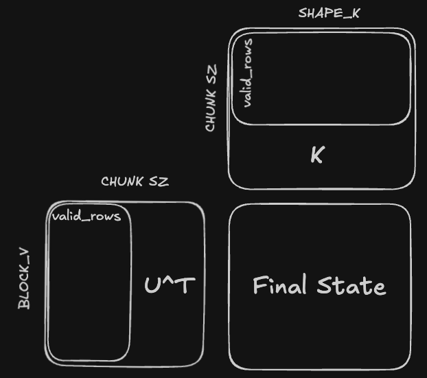
Chunked Sequential State Passing Kernel
I now move on to the second part of the forward pass, which is the sequential state passing kernel, illustrated in this nice image from the blog, as shown before:
The equation depicted is just the matrix version of the chunk-local state update equation with the $\mathbf{u,w}$ vectors: $$ \mathbf{S}^{r}_{[i]} = \mathbf{S}_{[i]} \left( \mathbf{I} - \sum_{t=1}^{r} \mathbf{w}_{[i]}^t \mathbf{k}_{[i]}^t \right) + \sum_{t=1}^{r} \mathbf{u}_{[i]}^t \mathbf{k}_{[i]}^t $$ This chunk-level equation is a significant improvement over its recurrent predecessor, but we still can't escape the sequential nature. This means that each SM in the kernel will need to compute the states over the entire sequence length, taking strides of $C$. I also wanted to include the final part of the forward pass, the Parallel Output Computation because of one specific multiplicand: the $\left(\mathbf{U_{[i]}} - \mathbf{W_{[i]}} \mathbf{S_{[i]}^T}\right)$ term. This term appears in the sequential state passing equation with some reorganization:
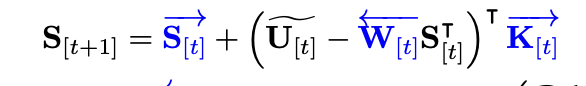
$$ \mathbf{S}_{[i+1]} = \mathbf{S}_{[i]} - \mathbf{S}_{[i]} \mathbf{W}_{[i]}^T \mathbf{K}_{[i]} + \mathbf{U}_{[i]}^T \mathbf{K}_{[i]} \newline = \mathbf{S}_{[i]} - (\mathbf{U_{[i]}} - \mathbf{W_{[i]}} \mathbf{S_{[i]}^T})^T \mathbf{K}_{[i]} $$
Thus, we can avoid recomputing this term in the Ouput computation kernel, since it is calculated as part of the sequential kernel, and the only extra step is adding a TMA store per chunk-step -- FLA also does this optimization. The issue lies in how to coordinate the different matmuls - the inner $\mathbf{W_{[i]}} \mathbf{S_{[i]}^T}$ matmul needs to accumulate into the $\mathbf{U_{[i]}}$ matrix, and the result then needs to be multiplied with the $\mathbf{K_{[i]}}$ matrix and accumulated into $\mathbf{S_{[i]}}$.
These define two distinct GEMM stages, each followed by a TMA store.
- The first stage is the accumulation into the $\mathbf{U_{[i]}}$ matrix, which then needs to be TMA stored back into GMEM.
- The second stage takes the result from the first stage, loades it into shared memory and performs another GEMM with $\mathbf{K_{[i]}}$ to compute the final state update, which gets accumulated into state registers that persist across chunk iterations.
- Finally, the chunk for the current state is updated and TMA stored, and on the next chunk iteration, the state registers need to be moved to SMEM to participate in the first GEMM.
You might notice there are several accumulations into registers in a single chunk iteration, and you might consider trying to replace a SS atom with a RS atom to avoid a RMEM -> SMEM store. I considered this as well, but because the $(\mathbf{U_{[i]}} - \mathbf{W_{[i]}} \mathbf{S_{[i]}^T})$ result needs to be transposed, this isn't possible, since $D$ layouts are always K-major, and the transpose creates a MN-layout, which RS does not support - the register operand must be in K-major for SM90.
Recurrent GDN Scheduler
So there are two different types of kernels in GDN forward passes - sequential and parallel, and each type requires its own scheduler. The RecurrentGDNScheduler is very similar to the previously covered ChunkGDNScheduler except it tiles over CTAs instead of SMs, and it doesn't distribute the $M$ dimension (sequence) across CTAs; each CTA needs to iterate over the entire sequence length.
Now the CTA tiling looks like this:
This tells us which portions of each of the matrices: $\mathbf{K_{[i]}}$, $\mathbf{W_{[i]}}$, $\mathbf{U_{[i]}}$, the current CTA reads - the state matrix is also further tiled along its rows dimension, so the CTA local state tensor is shape BLOCK_V $\times \mathbf{d_k}$, and I try to keep BLOCK_V greater than 64 if possible for Tensor Cores friendly shapes.
Here's the get_next_block function for RecurrentGDNScheduler, it's a little more compact than its ChunkGDNScheduler counterpart, since it doesn't need to split along the sequence dimension.
template <uint32_t BLOCK_V, uint32_t kNumVHeads, uint32_t kNumKHeads, uint32_t kNumBlocks, uint32_t kNumTMAMulticast>
struct RecurrentGDNScheduler {

  int shape_k, shape_v;
  int cur_block_idx;
  int current_iter = -1;
  int num_heads, batch_size, num_v_blocks;
  int num_blocks;
  bool is_valid_work = true;
  int actual_num_blocks;
  bool is_peer_cta_alive = true;

  __device__ __forceinline__ RecurrentGDNScheduler(int shape_v, int batch_size) {
    // calculate grid size and place them in a cluster together, so when writing partial sums it's easier to write
    // through
    this->shape_v = shape_v;
    this->batch_size = batch_size;
    this->num_v_blocks = ti_ceil_div(shape_v, BLOCK_V);
    // Store actual work items count before padding
    this->actual_num_blocks = num_v_blocks * kNumVHeads * batch_size;
    // Pad total work items to multiple of kNumTMAMulticast to ensure whole clusters stay alive
    this->num_blocks = ti_align(actual_num_blocks, kNumTMAMulticast);
  }

  __device__ __forceinline__ bool get_next_block(int &v_block_idx, int &v_head_idx, int &k_head_idx, int &batch_index) {
    // kNumBlocks is the total number of blocks allocated for this persistent scheduler
    // however, we can pack multiple head indices into the same SM
    cur_block_idx = (++current_iter) * kNumBlocks + blockIdx.x;

    if (cur_block_idx >= num_blocks) {
      return false;
    }
    // is_peer_cta_alive = (cur_block_idx ^ 1) < actual_num_blocks && same_seq_slab && same_k_head;
    v_head_idx = cur_block_idx % kNumVHeads;
    k_head_idx = (v_head_idx * kNumKHeads) / kNumVHeads; // equivalent to dividing by kNumTMAMulticast
    int v_head_blocked_idx = cur_block_idx / kNumVHeads;
    v_block_idx = v_head_blocked_idx % num_v_blocks;
    batch_index = v_head_blocked_idx / num_v_blocks;

    return true;
  }
}
All it does is determine the current batch index and head index the CTA is responsible for, since these are the only indices required to locate the current tile the SM is reponsible for. The total number of blocks is determined by the number of V heads, because Gated Delta Net actually Grouped Key + Query instead of Grouped Query, and the batch_size.
One last mention on indexing: because we're now using state tensors, which are stored at checkpoints of $C$, we have a new shape to deal with, which is $\left( B, \left \lceil S / C \right \rceil, d_v, d_k\right)$ for padded mode, and $\left (C', d_v, d_k \right)$ for varlen mode. $C' = \sum_{i=1}^{B} \left \lceil S_i / C \right \rceil$ is the total number of chunks across all batches, and it actually requires some host side computation, done by the prepare_cu_chunks function:
inline std::vector<int> prepare_cu_chunks(
  const std::vector<int>& cu_seqlens,
  int chunk_size = 64,
  bool output_final_state = false
) {
  alignas(8) std::vector<int> chunks(cu_seqlens.size() - 1); // batch_size
    for (int i = 1; i < cu_seqlens.size(); i++) {
        int length = cu_seqlens[i] - cu_seqlens[i-1];
        chunks[i - 1] = ti_ceil_div(length, chunk_size);
    }
  std::vector<int> cu_chunks; // (batch_size + 1)
  cu_chunks.push_back(0);
  int chunk_sum = 0;
  for (int i = 1; i < chunks.size() + 1; i++) {
    chunk_sum += chunks[i-1];
    cu_chunks.push_back(chunk_sum);
  }

  return cu_chunks;
}
Inputs
Here's the code for the TMA loads:
auto &barrier = tma_barrier_ws[0];
auto &barrier_k = tma_barrier_k[0];
// load the wS^T mma first, with reduction dimension SHAPE_V
if (chunk_idx == 0) {
tma_copy<SHAPE_K, BLOCK_V, kSwizzleSMode, __nv_bfloat16, 4>(&state_tensor_map, &barrier, sState, 0,
                                                            v_block_idx * BLOCK_V, 1, v_head_idx,
                                                            global_state_offset + chunk_idx);
}
tma_copy<SHAPE_K, kChunkSize, kSwizzleWMode, __nv_bfloat16, 4>(&w_tensor_map, &barrier, sW, 0, v_head_idx,
                                                                1, chunk_idx * kChunkSize, batch_index);
tma_copy<BLOCK_V, kChunkSize, kSwizzleUMode, __nv_bfloat16, 4>(
    &u_tensor_map, &barrier, sU, v_block_idx * BLOCK_V, v_head_idx, 1, chunk_idx * kChunkSize, batch_index);
(chunk_idx == 0) ? tma_barrier_ws[0].arrive_and_expect_tx(SMEM_STATE_SIZE_PER_STAGE + SMEM_U_SIZE_PER_STAGE +
                                                        SMEM_W_SIZE_PER_STAGE)
                : tma_barrier_ws[0].arrive_and_expect_tx(SMEM_U_SIZE_PER_STAGE + SMEM_W_SIZE_PER_STAGE);
tma_copy<SHAPE_K, kChunkSize, kSwizzleKMode, __nv_bfloat16, 4>(&k_tensor_map, &barrier_k, sK, 0, k_head_idx,
                                                                1, chunk_idx * kChunkSize, batch_index);
tma_barrier_k[0].arrive_and_expect_tx(SMEM_K_SIZE_PER_STAGE);
The matrices we load in, with their shapes are: $$ \mathbf{K_{[t]}} \in \mathbb{R}^{C \times b_k}, \mathbf{V_{[t]}} \in \mathbb{R}^{C \times b_v}, \mathbf{S_{[t]}} \in \mathbb{R}^{C \times d_v}, \mathbf{U_{[t]}} \in \mathbb{R}^{C \times b_v}, \mathbf{W_{[t]}} \in \mathbb{R}^{C \times d_k}, g_{[t]} \in \mathbb{R}^{C} $$ The state tensors are only loaded in on the first chunk index, since it is calculated recurrently. If no initial states exists, it is zero filled. Notice that there are two stages here - we first load in the required matrices for the first GEMM, and then we load in the $\mathbf{K_{[t]}}$ matrix by itself for the second GEMM. This was to reduce some of the TMA load overhead, but I'm not sure how much it actually helps without benchmarking. There's also further room for optimization with software pipelining, but I wanted to first get the code working.
GEMMs
First GEMM
Before the first WGMMA of $\mathbf{U}_{[t]} - \mathbf{W}_{[t]} \mathbf{S}_{[t]}^T$, the two GEMM accumulator registers, ws_accum and state_accum are initialized. ws_accum gets the initial values of U, and state_accum will get the initial values of state, if any exist.
load_swizzled_smem_to_accum<BLOCK_V, kChunkSize, kSwizzleUMode, WGMMA_M_PER_WARP>(sU, ws_accum, warpIdx,
                                                                                    lane_idx);
cutlass::arch::NamedBarrier::sync(kNumMathThreads, 1);
if (chunk_idx == 0) {
    if constexpr (!kIsInitialState) { // if we don't have an initial state, we force zero fill the state shared memory.
#pragma unroll
    for (int i = 0; i < STATE_MMA::kNumAccum; i++) {
        state_accum[i] = 0;
    }
    store_accum_to_swizzled_smem<SHAPE_K, BLOCK_V, kSwizzleSMode,
                                    WGMMA_M_PER_WARP>(state_accum, sState, warpIdx,
                                                    lane_idx);
    } else { // here we still need to perform a SMEM -> RMEM to get the initial state values in the accumulator registers
    load_swizzled_smem_to_accum<SHAPE_K, BLOCK_V, kSwizzleSMode,
                                WGMMA_M_PER_WARP>(sState, state_accum, warpIdx,
                                                    lane_idx);
    }
}
To keep the section concise, I'll show the base WGMMA descriptor creation and the looping logic, most of the other code is boilerplate:
using WSMMA = typename BF16MMASelector<BLOCK_V, Major::K, Major::K, cute::GMMA::ScaleIn::Neg>::type;
auto smem_w_desc = create_wgmma_desc<Major::K, kChunkSize, BLOCK_K, kSwizzleWMode>(sW); // (kChunkSize, BLOCK_K)
auto smem_state_desc = create_wgmma_desc<Major::K, BLOCK_V, BLOCK_K, kSwizzleSMode>(sState); // (BLOCK_V, BLOCK_K)

WSMMA::wgmma(smem_w_desc, smem_state_desc, ws_accum, 1);
Both descriptors are in K-major, since the reduction dimension is the key dimension, and the A scale for the WS WGMMA atom is negative one to ensure the WS term is negated when accumulating in. So this matches the $\mathbf{U}_{[t]} - \mathbf{W}_{[t]} \mathbf{S}_{[t]}^T$.
After the WS GEMM is finished, the now updated $\mathbf{U}_{[t]}$ needs to be stored back to global memory. FLA inserts a conditional flag for this store, but I think this is more for tweakability across their larger library - for a specialized GDN implementation it's a free optimization. The TMA store logic is identical to the previous UW kernel's, with one important difference when we store the final output state, which is part of the second GEMM.
The Ragged Varlen Output State Case
The final output state is important because it is the only 'memory' each GDN layer has about previous tokens, and it will be used in the decode stage to compute the next outputs. In the specific varlen scenario where the final state is being stored, but it is currently a ragged tile, this is what happens in the second GEMM $\mathbf{S}_{[i]} - \left (\mathbf {U'_{[i]}} \right )^T \mathbf{K}_{[i]}$:
The second GEMM's reduction dimension is the sequence dimension, so if the kernel is in a sequence that is NOT the last sequence, and the current sequence length is NOT a multiple of the chunk size $C$, the TMA load will still pull in a full $C$ rows on the last chunk of this sequence. For example, if the current sequence length is 113, and $C = 64$, the TMA load will pull in 64 rows, but only 53 of them will be used, and the remaining 11 rows actually be the next sequence's first chunk.
This pollutes the results of the final output state, and the fix is to zero out the accumulator registers and then store into SMEM for the second GEMM.
For the updated $\mathbf{U'_{[i]}}$ matrix, all this requires is a small check, since the registers are already loaded in:
#pragma unroll
for (int val_idx = 0; val_idx < WSMMA::kNumAccum; val_idx++) {
    auto [row_idx, col_idx] = get_accum_row_col(threadIdx.x, val_idx);
    bool pred = global_row_offset + row_idx < seq_end;
    // include this to zero out the U tensor on ragged tiles for downstream computation
    if constexpr (kOutputFinalState) {
        if (!pred) {
            ws_accum[val_idx] = 0.f;
       }
    }
}
For the $\mathbf{K_{[i]}}$ matrix, we use the same logic, but the registers need to be loaded from SMEM:
bool full_chunk = global_row_offset + kChunkSize - 1 < seq_end; // check if the current chunk is a full chunk for ragged tiles
if constexpr (kIsVarLen && kOutputFinalState) {
    // zero out the K tensor on ragged tiles, and store back
    // so this ensures that the rows are zeroed out for ragged tiles for the A operand
    if (!full_chunk) {
        if constexpr (!kUseGate)
        store_accum_to_swizzled_smem<BLOCK_V, kChunkSize, kSwizzleUMode, WGMMA_M_PER_WARP>(ws_accum, sU, warpIdx,
                                                                                                 lane_idx);
    // we now need to ensure for K that they are zeroed out
    constexpr int kNumMathWarps = kNumMathThreads / 32;
    float sK_accum[SHAPE_K / 2]; // N / 2 number of values, since there's 4 registers per 8 columns
    load_swizzled_smem_to_accum<SHAPE_K, kChunkSize, kSwizzleKMode, WGMMA_M_PER_WARP>(sK, sK_accum, warpIdx,
                                                                                        lane_idx);
#pragma unroll
    for (int val_idx = 0; val_idx < SHAPE_K / 8; val_idx++) {
        const auto [row_idx, col_idx] = get_accum_row_col(threadIdx.x, val_idx);
        bool pred = global_row_offset + row_idx < seq_end;
        if (!pred) {
        sK_accum[val_idx] = 0.f;
        }
    }
    store_accum_to_swizzled_smem<SHAPE_K, kChunkSize, kSwizzleKMode, WGMMA_M_PER_WARP>(sK_accum, sK, warpIdx,
                                                                                        lane_idx);
    cutlass::arch::NamedBarrier::sync(kNumMathThreads, 1);
    }
}
Once the appropriate rows in the $\mathbf{K_{[i]}}$ matrix are zeroed out, the updated values are stored back into SMEM, and similarly for the $\mathbf{U_{[i]}}$ matrix, which was already zeroed out in the ragged store. You'll notice that when gating is turned off, the kernel doesn't actually need to store back the U matrix. Let's look at the gating section next.
Gating Term
  if constexpr (kUseGate) {
// now that V is fully updated, we multiply the V with the gate values
#pragma unroll
for (int val_idx = 0; val_idx < WSMMA::kNumAccum; val_idx++) {
    auto [row_idx, col_idx] = get_accum_row_col(threadIdx.x, val_idx);
    bool pred = global_row_offset + row_idx < seq_end;
    if (pred) {
        ws_accum[val_idx] *= __expf(gate_last - s_gate[row_idx]); // gating decay
    }
}
gate_last = __expf(gate_last);

#pragma unroll
for (int i = 0; i < STATE_MMA::kNumAccum; i++) {
    state_accum[i] *= gate_last; // gating decay
}
// Wait for the TMA store of pre-gating sU to finish reading smem before we overwrite
if (warpIdx == 0) {
    cute::tma_store_wait<0>();
}
cutlass::arch::NamedBarrier::sync(kNumMathThreads, 1);

// Write gated ws_accum back to sU so the outer SS WGMMA reads gated values
store_accum_to_swizzled_smem<BLOCK_V, kChunkSize, kSwizzleUMode, WGMMA_M_PER_WARP>(ws_accum, sU, warpIdx,
                                                                                    lane_idx);
cutlass::arch::NamedBarrier::sync(kNumMathThreads, 1);
}
Once gating is introduced though, the ragged varlen case gets a lot more interesting. I'm going to first outline the problem at hand, and then list the different paths that can be done to handle both ragged varlen and gating, and then what I ended up doing. This is the fun part of kernel engineering - when the decision space grows to more than a couple decisions and you need to start thinking about how to neatly deal with all the problems, while maintaining performance.
This gating section is actually applying the gate terms to the $\mathbf{K_{[t]}}$, but it's multipling the gates on the new $\mathbf{U_{[t]}}$ result. Why? Well, if we look at a snapshot of the paper's equations:

It's because the rows of $\mathbf{U_{[t]}}$, when transposed are the reduction dimension in the GEMM shown above, and they multiply with the rows of $\mathbf{K}_{[t]}$, so applying the gating term on either the rows of etiher matrix is equivalent. This is what FLA does, but the TMA store of U in the middle of the two GEMMs now complicates things, since we're storing the non-gated $\mathbf{U_{[t]}}$ matrix back into global memory for the next kernel. This means when gating is turned off, the entire kernel needs to wait for the U store to finish to apply the gating terms.
The other option is to load the $\mathbf{K_{[t]}}$ tile in shared memory into the registers, and apply the gating term to its rows, then store back to shared memory. This is nice because we already do this on ragged varlen output tiles - however that's the ONLY time we need to do this load-store. Otherwise on any other varlen or padded tile it's unnecessary since the ws_accum registers are readily available to apply gating. Furthermore, when gating we already store ws_accum back to shared memory every iteration, saving another unnecessary store if gating on K.
Still, the TMA store remains an issue for the first option, because once we update the $\mathbf{U_{[t]}}$ with gating terms, we need to writeback to the sU tile, and this means blocking on completion of the previous tma store so we don't corrupt memory in transit or waiting to be read.
I put a small analysis in the epilogue with some benchmarking - look in the Appendix for further informations. The analysis shows that the second kernel is faster across all test cases. This makes sense since Kernel 1's issuing and blocking on the TMA store eats far more cycles compared to doing a 'ld.sync' and 'st.sync' in Kernel 2, even when gating is turned and the stores become unnecessary. So I chose to go with Kernel 2, but kept both kernels (they're only different by a few lines) in the repository for reference.
Chunked Output Computation
Almost to the end! This is the final kernel in the forward pass, and it also shows the power of linear attention in full force. Let's first copy down the equation again: $$ \mathbf{O_{[t]}} = \mathbf{Q}_{[t]} \mathbf{S}_{[t]}^T + (\mathbf{Q}_{[t]} \mathbf{K}_{[t]}^T \odot \mathbf{\Gamma_{[t]}}) \mathbf{V}_{[t]} $$
There's two distinct computations here - the first is the $\mathbf{Q}_{[t]} \mathbf{S}_{[t]}$ matrix multiplication, and the second is the $(\mathbf{Q}_{[t]} \mathbf{K}_{[t]}^T \odot \mathbf{\Gamma_{[t]}}) \mathbf{V}_{[t]}$ matrix multiplication. For the latter GEMM, it contains a similar structure to the double GEMM in the sequential state passing kernel, where the second stage of the GEMM depends on the outputs of the first stage.
Because of this structure, $\mathbf{K_{[t]}}$ matrix is tiled across both of its dimensions, since both its $M$ and $K$ dimensions will be matrix reduction dimensions:
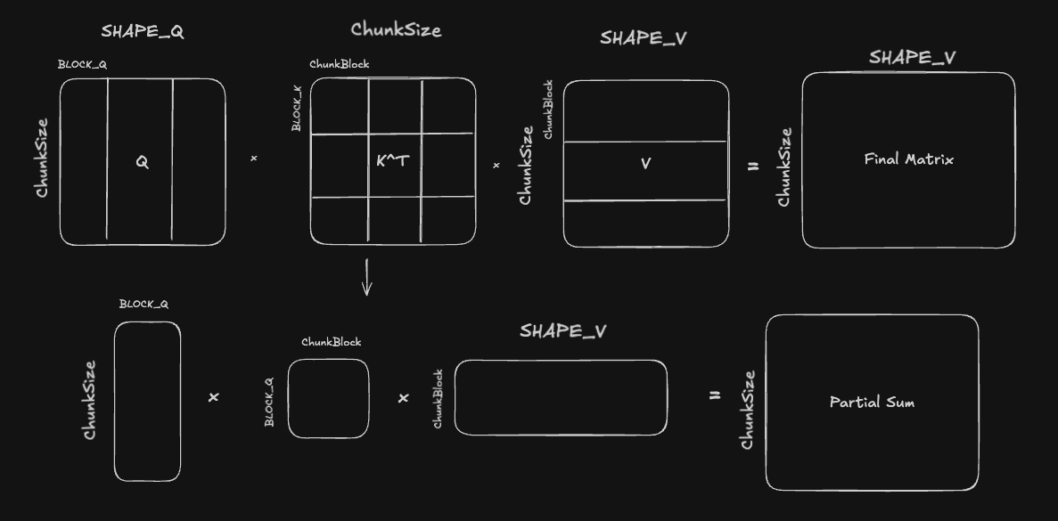
Although it looks like SHAPE Q/K/V are all different because of notation, Q and K should obviously always have the same shape, but it is also valid to make the assumption that SHAPE Q = SHAPE V - FLA does this, and most GDN configs I've seen online do this as well.
The naive approach for two conseuctive GEMMs would be to fully complete the $\mathbf{Q}_{[t]} \mathbf{K_{[t]}}^T$ matmul, and then multiply the result with the $\mathbf{V_{[t]}}$ matrix. This would require explicit warpgroup sychronization after the first GEMM, and we would also be loading $\mathbf{V_{[t]}}$ from global memory without using it for a while, wasting bandwidth.
There are multiple beneifts to using this double tiling approach for the intermediate, shared matrix:
- Instead of waiting for the entire first GEMM to finish, only the first 'skinny GEMM' needs to be completed, which will complete faster because of its smaller K dimension.
- Instead of the number of pipelining stages being limited to (SHAPE K) / (BLOCK K), we can now pipeline across both SHAPE K and ChunkSize dimensions, allowing more oppportunities to hide latency.
- It's easier to tune shared memory usage across different problem sizes, because we can tune both the number of stages and the BLOCK K, ChunkBlock dimensions independently, depending on which dimension is larger.
TMA Copies
As always, let's start with the TMA copies, and only at the varlen case, since the padded case is similar.
constexpr uint32_t num_k1_blocks = SHAPE_K / BLOCK_K;
constexpr uint32_t num_k2_blocks = kChunkShape / kChunkBlock;
for (int k2_block_idx = 0; k2_block_idx < num_k2_blocks; ++k2_block_idx) {
    for (int k1_block_idx = 0; k1_block_idx < num_k1_blocks; ++k1_block_idx) {
    math_barriers[stage_idx]->wait(phase ^ 1);
    auto barrier = tma_barriers[stage_idx];
    // we group the Q, S matrix loads together since they're only done on the first iteration
    // however, we need to use a different stage idx for these shared memory loads, to avoid
    if (k2_block_idx == 0) {
        tma_copy<BLOCK_K, BLOCK_V, kSwizzleSMode, __nv_bfloat16, 4>(&state_tensor_map, barrier, sState[stage_idx],
                                                                    k1_block_idx * BLOCK_K, v_block_idx * BLOCK_V,
                                                                    1, v_head_idx, global_state_offset);
    }
    tma_copy<BLOCK_K, kChunkShape, kSwizzleQMode, __nv_bfloat16, 3>(
        &q_tensor_map, barrier, sQ[stage_idx], k1_block_idx * BLOCK_K, k_head_idx, 1, global_row_offset);
        // copy K
    tma_copy<BLOCK_K, kChunkBlock, kSwizzleKMode, __nv_bfloat16, 3>(
        &k_tensor_map, barrier, sK[stage_idx], k1_block_idx * BLOCK_K, k_head_idx, 1,
        global_row_offset + k2_block_idx * kChunkBlock);
    tma_copy<BLOCK_V, kChunkBlock, kSwizzleUMode, __nv_bfloat16, 3>(
        &u_tensor_map, barrier, sU[stage_idx], v_block_idx * BLOCK_V, v_head_idx, 1,
        global_row_offset + k2_block_idx * kChunkBlock);
    if (k2_block_idx == 0) {
        tma_barriers[stage_idx]->arrive_and_expect_tx(SMEM_STATE_SIZE_PER_STAGE + SMEM_K_SIZE_PER_STAGE +
                                                    SMEM_Q_SIZE_PER_STAGE + SMEM_U_SIZE_PER_STAGE);
    } else {
        tma_barriers[stage_idx]->arrive_and_expect_tx(SMEM_U_SIZE_PER_STAGE + SMEM_K_SIZE_PER_STAGE +
                                                    SMEM_Q_SIZE_PER_STAGE);
    }

    advance_pipeline();
    }
}
The inner loop loops over the head dimension, which is the reduction dimension for the $\mathbf{Q}_{[t]} \mathbf{K_{[t]}}^T = \mathbf{P_{[t]}}, \mathbf{Q}_{[t]} \mathbf{S}_{[t]}^T$ GEMMs, and the outer loop loops over the chunk (sequence) dimension, which is the reduction dimension for the $(\mathbf{P_{[t]}} \odot \mathbf{\Gamma_{[t]}}) \mathbf{V_{[t]}}$ matmul. You'll notice that the $\mathbf{S_{[t]}}$ matrix is only loaded in on the first iteration of the outer loop, since it's only needed for the first GEMM, but the $\mathbf{Q_{[t]}}$ matrix is loaded across both loops.
This is a redundant load, since the $\mathbf{Q_{[t]}}$ tile coordinates don't depend on k2_block_idx, so the kernel is loading the same tile across k2_block_idx iterations. However, it is an operand in the k2_block_idx loop, so the stage it writes to, sQ[stage_idx] needs to stay in sync with sK[stage_idx] which does change between both loops. Same reasoning for the $\mathbf{U_{[t]}}$ matrix, which is meant to replace the $\mathbf{V_{[t]}}$ matrix in the equation.
I don't love that this is the solution I came to -- an alternate solution is to load in the $\mathbf{Q_{[t]}}, \mathbf{U_{[t]}}$ matrices statically before this loop, so that the kernel doesn't depend on the stage_idx variable as the index. But this then fails to take advantage of the pipelining. I think this problem is heavily dependent on the shapes given to the kernel, like a larger kChunkSize over the sequence dimension means a higher num_k2_blocks, thus more redunancy with the Q and S loads. This would appear in Blackwell, where the GEMM M = 128. Nevertheless, it's a really interesting optimization problem that I'm sure smarter people than me have tackled, so further research (maybe another writeup) is warranted.
The GEMMs
I'm going to skip over the $\mathbf{Q_{[t]} \mathbf{S}_{[t]}^T}$ GEMM, since at this point it's a pattern already covered. Let's look at the full second GEMM instead, across all three matrices:
auto smem_q_desc = create_wgmma_desc<Major::K, kChunkShape, BLOCK_K, kSwizzleQMode>(sQ[stage_idx]);
auto smem_k_desc = create_wgmma_desc<Major::K, kChunkBlock, BLOCK_K, kSwizzleKMode>(sK[stage_idx]);
#pragma unroll
for (int k = 0; k < BLOCK_K / QK_MMA::K; k++) {
    QK_MMA::wgmma(smem_q_desc, smem_k_desc, QKT_accum, k);
}
cute::warpgroup_commit_batch();
#pragma unroll
for (int i = 0; i < QK_MMA::kNumAccum; i++) {
    auto [row_idx, col_idx] = get_accum_row_col(threadIdx.x, i);
    // remember k2_block_idx = kChunkShape / kChunkBlock, and tells us the column offset in P
    int global_col = col_idx + k2_block_idx * kChunkBlock;
    bool valid = row_idx >= global_col;
    if (seq_end_in_chunk >= 0) {
            valid &= (row_idx <= seq_end_in_chunk) && (global_col <= seq_end_in_chunk);
    }
    float gate_val = 1.0f;
    if constexpr (kUseGating) {
        gate_val = __expf(s_gate[row_idx] - s_gate[global_col]);
    }
    QKT_accum_bf16[i] =
        valid ? __float2bfloat16_rn(QKT_accum[i] * scale_factor * gate_val) : __nv_bfloat16(0.0f);
}
I've stripped out the WGMMA boilerplate again, but after the first wgmma, each value in QKT_accum now contains a partial sum of $\mathbf{P_{[t]}}$, the temporary matrix. We then need to perform the causal gate masking, where for each value we fetch the row and the global column of $\mathbf{P_{[t]}}$, and check the lower diagonal condition, and additionally a bounds mask if in a ragged tile. The elementwise gating mask $\mathbf{\Gamma_{[t]}}$ is also applied, and a scale factor of $\frac{1}{\sqrt{d_k}}$, similar to vanilla attention.
The second GEMM, $\mathbf{P_{[t]}} \mathbf{U_{[t]}}$:
auto smem_u_desc = create_wgmma_desc<Major::MN, BLOCK_V, kChunkBlock, kSwizzleUMode>(sU[stage_idx]);
#pragma unroll
for (int k = 0; k < kChunkBlock / PU_MMA::K; k++) {
    __nv_bfloat16 *shifted_QKT_accum = QKT_accum_bf16 + k * 8;
    uint32_t *packed_accum = reinterpret_cast<uint32_t *>(shifted_QKT_accum);
    PU_MMA::wgmma(packed_accum[0], packed_accum[1], packed_accum[2], packed_accum[3], smem_u_desc, PU_accum, 1);
}
cute::warpgroup_commit_batch();
Since the partial accumulations of QKT are persisted through register memory, I can use the RS (Register + Shared) WGMMA instruction to avoid storing back the A operand into shared memory.
The GEMMs are repeated across the num_k1_blocks and num_k2_blocks loops, and at the end there is one final accumulation (and gating step) that we need to do to get $\mathbf{O_{[t]}} = \mathbf{Q_{[t]}} \mathbf{S_{[t]}}^T + (\mathbf{Q_{[t]}} \mathbf{K_{[t]}}^T \odot \mathbf{\Gamma_{[t]}}) \mathbf{V_{[t]}}$:
float gate_val = 1.0f;
#pragma unroll
for (int i = 0; i < PU_MMA::kNumAccum; i++) {
    if constexpr (kUseGating) {
        auto [row, col] = get_accum_row_col(threadIdx.x, i);
        gate_val = __expf(s_gate[row]);
    }
    QS_accum[i] = gate_val * QS_accum[i] * scale_factor + PU_accum[i];
}
The QS_accum was the accumulator registers for the $\mathbf{Q_{[i]}} \mathbf{S_{[i]}}^T$ GEMM I chose to omit, and remember that the $\mathbf{Q_{[i]}}$ has its own row-wise gating term (look at the paper snapshot above for reference). Then we obviously store from RMEM to SMEM, and then initiate a TMA store to GMEM for the final result.
Comparison with FLA
Speedup with FLA
The kernels achieve parity with the FLA Triton implementation on the shapes listed in the repository. I also benchmarked the first round of unoptimized kernels, that were built for correctness - see the appendix for the full table. I noticed my implementation beat FLA on the smaller batch shapes, but on the larger batch shapes with more rows, it does much poorly - up to 0.45x slower than FLA for some shapes. I think the primary reason for this slowdown is that each SM receives more work blocks from the persistent scheduler, and the pipeline bubbles where the tensor cores idle builds up across persistent iterations. Pingpong scheduling should fix this.
Turning on FLA's FLA_USE_CUDA_GRAPH to turn on cuda graphs in the @triton.autotune decorates gives an even bigger speedup to the FLA side, without an equivalent speedup in my implementation. I'm not entirely sure why this happens since I don't have enough experience with CUDA graphs - Opus said that it's most likely due to the preprocessing transpose kernels and some expensive host side allocations using libtorch.
To get around this, we could build up a 'shape cache' that is similar in spirit to a JIT cache, but lazy allocates tensor memory for the first time a new shape is encountered, and continues to use this tensor until the next shape is encountered. I started writing a first try of this in the repository, under the separate branch 'prealloc_workspace_exp'. Another option is to allocate large 'fake' tensors, like a lot of inference libraries do to further avoid any host side allocations and always use a fixed tensor.
A Note on Padding
One last note on padding, which I had to write after completing the kernels and was testing parity with FLA. Until then, I had only set up the JIT launchers for each kernel to handle nice head dimensions that were multiples of 32 or 64 to maximize swizzling, but the FLA tests contained head dimensions of 60 and 120. The fix was to add an alignment check with libtorch's zero pad method - on some edge cases this can hamper performance a good bit, but I think most reasonable model architectures are using 64-multiple head dimensions to be hardware aware - no reason not to. The only issue is that the torch.pad method is inefficient, since it allocates a new tensor and copies the data over.
Wrap-Up
This is my full thought process behind writing a fully CUDA implementation of the GDN prefill forward pass on SM90. Curious readers might now be wondering why I haven't mentioned the recurrent kernel. Because it is a much simpler kernel and equation involving three GEMVs, the technical details are not as interesting as the coordination of GEMMs and pipelining for prefill - I provided an implementation in the repository.
Next Steps
Performance Improvements
For next steps, I would love to get my hands on some Blackwell GPUs to use 2SM MMAs and CLCs for better performance. I think 2CTA is especially necessary for head dim = 256, since you could do 128 x 256 shapes for especially large prefill workloads. For the compute O kernel, experimenting with deeper pipelines between TMA and GEMM and intra-GEMM is worthwhile as well as seeing if first fully computing the $\mathbf{Q_{[t]}} \mathbf{K_{[t]}}^T \odot \mathbf{\Gamma_{[t]}}$ term is better for some shapes.
There's also plenty of performance left to squeeze out of these kernels on SM90, I think a straightforward next step would be to implement consumer warpgroup pingpong scheduling. I'm relatively confident this will give the most performance gains out of any next step, because the first two kernels in the forward pass have two GEMMs right after each other, but with some nontrivial gating logic that leaves the Tensor Cores idle -- like the large TMA of $\mathbf{U_{[t]}}$ inside the sequential state update kernel, and the forward substition logic inside the compute UW kernel. Ping pong scheduling is the exact solution for this, since two consumer warpgroups can alternate in handling the ALU intensive arithmetic and loads while the other keeps the Tensor Cores busy.
Further, I definitely want to try ThunderKittens to rewrite all of the kernels, as well as for any further optimizations. I'm currently learning it to optimize FP8 MoE kernels, and I think it would make the kernels more readable but importantly increase iteration speed by a good amount.
More Parity with FLA
To actually get the full GDN forward pass, you do need to perform a L2 normalization on the QK vectors - this should be a pretty straightforward kernel that can be JITted, but I want to move on to MoE kernels, so these changes are open for grabs.
Appendix:
Stmatrix + Ldmatrix wrappers
With how often I used both the stmatrix.sync and ldmatrix.sync PTX instructions, I wrote wrappers for the swizzling logic used before the instructions, based off of DeepGEMM's code. Before we issue the actual stores/loads, there's a two stage swizzling operation that needs to be done to avoid bank conflicts and match the swizzling layout that the TMA store atom expects.
The first swizzle operation is to map the current tile of $\left( 64 \times \text{bN} / 8 \right)$ WGMMA output elements to the kSwizzleMode from the Tensor Map, and the second operation does another set swizzle of 128B to avoid shared memory bank conflicts. The second swizzle operator is the canonical 128B defined by CuTE : $\text{Swizzle} <3, 4, 3>$. See the swizzling section in Modular's blog for some intuition and great diagrams. The CuTLASS repo's swizzle.hpp also has clear comments.
Note that both the store and load methods are only converting between BF16 and FP32 - other conversions on newer architecture require some rewrites, especially for TMEM on >= SM100. But the core idea remains the same.
// Store float accumulator registers as bf16 to swizzled shared memory.
// Handles multiple swizzle atoms when BLOCK_INNER > swizzle_atom_size.
// Template params:
//   BLOCK_INNER: number of elements in the inner (N/V) dimension
//   BLOCK_OUTER: number of elements in the outer (M) dimension (for atom stride calculation)
//   kSwizzleMode: swizzle mode in bytes (0 for non-swizzled, 32/64/128 for swizzled)
//   WGMMA_M_PER_WARP: rows per warp (typically MMA::M / 4 = 16)
template <uint32_t BLOCK_INNER, uint32_t BLOCK_OUTER, uint32_t kSwizzleMode, uint32_t WGMMA_M_PER_WARP>
__device__ __forceinline__ void store_accum_to_swizzled_smem(float *accum, __nv_bfloat16 *smem_ptr, int warp_idx,
                                                             int lane_idx) {
  constexpr uint32_t kNumBankGroupBytes = 16;
  constexpr uint32_t kNumIter = BLOCK_INNER / 8; // Each iteration handles 8 elements (4 accum values * 2 bf16)
#pragma unroll
  for (int i = 0; i < kNumIter; i++) {
    uint8_t *ptr = nullptr;
    if constexpr (kSwizzleMode > 0) {
      constexpr uint32_t kSwizzleAtomSize = kSwizzleMode / sizeof(__nv_bfloat16); // elements per swizzle atom
      int atom_offset = i / (kSwizzleAtomSize / 8);
      int in_atom_offset = i % (kSwizzleAtomSize / 8);
      int bank_group_index = in_atom_offset + lane_idx * (kSwizzleMode / kNumBankGroupBytes);
      int row = bank_group_index / 8, col = bank_group_index % 8;
      col ^= row % (kSwizzleMode / 16); //
      ptr = reinterpret_cast<uint8_t *>(smem_ptr) + atom_offset * BLOCK_OUTER * kSwizzleMode +
            WGMMA_M_PER_WARP * kSwizzleMode * warp_idx + row * (kNumBankGroupBytes * 8) + col * kNumBankGroupBytes;
    } else {
      ptr = reinterpret_cast<uint8_t *>(smem_ptr + (WGMMA_M_PER_WARP * warp_idx + lane_idx) * BLOCK_INNER + i * 8);
    }
    custom_SM90_U32x2_STSM_N<__nv_bfloat162>::copy(__float22bfloat162_rn({accum[i * 4 + 0], accum[i * 4 + 1]}),
                                                   __float22bfloat162_rn({accum[i * 4 + 2], accum[i * 4 + 3]}), ptr);
  }
  cute::tma_store_fence(); // memory fence to ensure writes are visible after this point
}

// Load bf16 data from swizzled shared memory into float accumulator registers.
// This assumes a single swizzle atom (BLOCK_INNER * sizeof(bf16) == kSwizzleMode for K-major layouts).
// Template params:
//   BLOCK_INNER: number of elements in the inner (K) dimension
//   kSwizzleMode: swizzle mode in bytes (0 for non-swizzled, 32/64/128 for swizzled)
//   WGMMA_M_PER_WARP: rows per warp (typically MMA::M / 4 = 16)
template <uint32_t BLOCK_INNER, uint32_t BLOCK_OUTER, uint32_t kSwizzleMode, uint32_t WGMMA_M_PER_WARP>
__device__ __forceinline__ void load_swizzled_smem_to_accum(__nv_bfloat16 *smem_ptr, float *accum, int warp_idx,
                                                            int lane_idx) {
  constexpr uint32_t kNumBankGroupBytes = 16;
#pragma unroll
  for (int col_idx = 0; col_idx < BLOCK_INNER / 8; col_idx++) {
    float *shifted_accum = accum + col_idx * 4;
    uint8_t *ptr = nullptr;
    if constexpr (kSwizzleMode > 0) {
      constexpr uint32_t kSwizzleAtomSize = kSwizzleMode / sizeof(__nv_bfloat16); // elements per swizzle atom
      int atom_offset = col_idx / (kSwizzleAtomSize / 8);
      int in_atom_offset = col_idx % (kSwizzleAtomSize / 8);
      int bank_group_index = in_atom_offset + lane_idx * (kSwizzleMode / kNumBankGroupBytes);
      int row = bank_group_index / 8, col = bank_group_index % 8;
      col ^= row % (kSwizzleMode / 16);
      // Reshape layout from (BLOCK_M, kSwizzleMode / kNumBankGroupBytes) to
      // (BLOCK_M * kSwizzleMode / kNumBankGroupBytes / 8, 8) to match TMA 128B line layout
      ptr = reinterpret_cast<uint8_t *>(smem_ptr) + WGMMA_M_PER_WARP * warp_idx * kSwizzleMode +
            atom_offset * BLOCK_OUTER * kSwizzleMode + row * (kNumBankGroupBytes * 8) + col * kNumBankGroupBytes;
    } else {
      ptr =
          reinterpret_cast<uint8_t *>(smem_ptr + (WGMMA_M_PER_WARP * warp_idx + lane_idx) * BLOCK_INNER + col_idx * 8);
    }
    const uint2 data = custom_SM90_U32x2_STLM_N::load(ptr);
    __nv_bfloat162 bf16_pair1 = *reinterpret_cast<const __nv_bfloat162 *>(&data.x);
    __nv_bfloat162 bf16_pair2 = *reinterpret_cast<const __nv_bfloat162 *>(&data.y);

    shifted_accum[0] = __bfloat162float(bf16_pair1.x);
    shifted_accum[1] = __bfloat162float(bf16_pair1.y);
    shifted_accum[2] = __bfloat162float(bf16_pair2.x);
    shifted_accum[3] = __bfloat162float(bf16_pair2.y);
  }
}
Seq State Update Performance Analysis
I ran a quick benchmarking comparison between the two different possible kernels - labeled seq state update 1 and 2, for the first and second methods described in the Seq State section above. Seq state update 1 / 2 ratios - a higher ratio means that Kernel 1 took longer by that amount - so Kernel 2 is faster across all test cases.
| Mode | Shape Case | Latency Ratio (Median) | Latency Ratio (P95) | Latency Ratio (Min) | Latency Ratio (Max) |
|---|---|---|---|---|---|
| padded | B=1,T=63,H=1,D=64,gate_norm=1.0,mask_p=0.0 | 2.93x | 2.65x | 3.08x | 3.03x |
| padded | B=2,T=500,H=3,D=60,gate_norm=1.0,mask_p=0.0 | 2.74x | 2.71x | 2.64x | 2.82x |
| padded | B=2,T=1000,H=3,D=64,gate_norm=1.0,mask_p=0.5 | 2.00x | 1.96x | 2.08x | 2.18x |
| padded | B=3,T=1024,H=4,D=100,gate_norm=0.1,mask_p=0.0 | 1.92x | 2.09x | 1.81x | 43.32x |
| padded | B=4,T=1024,H=4,D=128,gate_norm=1.0,mask_p=0.0 | 1.66x | 1.64x | 1.66x | 1.80x |
| padded | B=2,T=1500,H=4,D=128,gate_norm=10.0,mask_p=0.0 | 1.66x | 1.64x | 1.66x | 1.73x |
| padded | B=4,T=2048,H=8,D=64,gate_norm=1.0,mask_p=0.0 | 1.95x | 1.95x | 1.98x | 2.02x |
| padded | B=8,T=512,H=8,D=64,gate_norm=1.0,mask_p=0.0 | 2.06x | 2.11x | 2.13x | 2.26x |
| padded | B=16,T=512,H=8,D=64,gate_norm=1.0,mask_p=0.0 | 1.80x | 1.85x | 1.79x | 1.89x |
| padded | B=32,T=256,H=8,D=64,gate_norm=1.0,mask_p=0.0 | 1.75x | 1.71x | 1.79x | 1.89x |
| padded | B=64,T=128,H=8,D=64,gate_norm=1.0,mask_p=0.0 | 1.58x | 1.67x | 1.65x | 1.77x |
| padded | B=8,T=512,H=8,D=128,gate_norm=1.0,mask_p=0.0 | 1.29x | 1.31x | 1.29x | 1.38x |
| padded | B=16,T=256,H=8,D=128,gate_norm=1.0,mask_p=0.0 | 1.34x | 1.33x | 1.35x | 1.40x |
| padded | B=32,T=128,H=8,D=128,gate_norm=1.0,mask_p=0.0 | 1.24x | 1.27x | 1.23x | 1.29x |
| padded | B=64,T=64,H=8,D=128,gate_norm=1.0,mask_p=0.0 | 1.14x | 1.10x | 1.17x | 1.30x |
| varlen | B=1,total_tokens=15,H=4,D=60,mask_p=0.0 | 1.78x | 1.72x | 1.78x | 1.49x |
| varlen | B=3,total_tokens=1000,H=4,D=64,mask_p=0.0 | 1.65x | 1.65x | 1.74x | 1.70x |
| varlen | B=3,total_tokens=1000,H=4,D=64,mask_p=0.5 | 1.65x | 1.65x | 1.74x | 1.76x |
| varlen | B=5,total_tokens=2000,H=4,D=100,mask_p=0.0 | 1.48x | 1.56x | 1.46x | 1.75x |
| varlen | B=1,total_tokens=8192,H=4,D=60,mask_p=0.0 | 1.86x | 1.86x | 1.84x | 1.95x |
| varlen | B=8,total_tokens=4096,H=4,D=64,mask_p=0.0 | 1.78x | 1.74x | 1.78x | 1.84x |
| varlen | B=16,total_tokens=8192,H=4,D=64,mask_p=0.0 | 1.78x | 1.65x | 1.78x | 1.84x |
| varlen | B=32,total_tokens=8192,H=4,D=64,mask_p=0.0 | 1.77x | 1.77x | 1.75x | 1.39x |
| varlen | B=64,total_tokens=8192,H=4,D=64,mask_p=0.0 | 1.77x | 1.63x | 2.00x | 1.91x |
| varlen | B=32,total_tokens=4096,H=4,D=128,mask_p=0.0 | 1.72x | 1.52x | 1.71x | 1.54x |
| varlen | B=64,total_tokens=6656,H=4,D=128,mask_p=0.0 | 1.33x | 1.32x | 1.33x | 1.36x |
| varlen | B=128,total_tokens=4608,H=4,D=64,mask_p=0.5 | 1.77x | 1.72x | 1.88x | 1.50x |
Latency results and speedup (FLA/gdn_cuda):
| Mode | Shape Case | Speedup (Median) | Speedup (P95) | Speedup (Min) | Speedup (Max) |
|---|---|---|---|---|---|
| padded | B=1,T=63,H=1,D=64,gate_norm=1.0,mask_p=0.0 | 3.22× | 3.44× | 3.14× | 3.10× |
| padded | B=2,T=500,H=3,D=60,gate_norm=1.0,mask_p=0.0 | 2.35× | 2.56× | 2.23× | 2.86× |
| padded | B=2,T=1000,H=3,D=64,gate_norm=1.0,mask_p=0.5 | 2.44× | 2.68× | 2.35× | 2.28× |
| padded | B=3,T=1024,H=4,D=100,gate_norm=0.1,mask_p=0.0 | 1.09× | 1.18× | 1.06× | 1.22× |
| padded | B=4,T=1024,H=4,D=128,gate_norm=1.0,mask_p=0.0 | 1.23× | 1.37× | 1.19× | 2.08× |
| padded | B=2,T=1500,H=4,D=128,gate_norm=10.0,mask_p=0.0 | 1.18× | 1.28× | 1.14× | 1.25× |
| padded | B=4,T=2048,H=8,D=64,gate_norm=1.0,mask_p=0.0 | 0.45× | 0.48× | 0.43× | 0.52× |
| padded | B=8,T=512,H=8,D=64,gate_norm=1.0,mask_p=0.0 | 0.86× | 0.95× | 0.83× | 1.28× |
| padded | B=16,T=512,H=8,D=64,gate_norm=1.0,mask_p=0.0 | 0.48× | 0.51× | 0.46× | 0.53× |
| padded | B=32,T=256,H=8,D=64,gate_norm=1.0,mask_p=0.0 | 0.48× | 0.51× | 0.46× | 0.77× |
| padded | B=64,T=128,H=8,D=64,gate_norm=1.0,mask_p=0.0 | 0.47× | 0.53× | 0.45× | 6.77× |
| padded | B=8,T=512,H=8,D=128,gate_norm=1.0,mask_p=0.0 | 0.80× | 0.89× | 0.77× | 1.18× |
| padded | B=16,T=256,H=8,D=128,gate_norm=1.0,mask_p=0.0 | 0.80× | 0.86× | 0.77× | 1.82× |
| padded | B=32,T=128,H=8,D=128,gate_norm=1.0,mask_p=0.0 | 0.77× | 0.81× | 0.75× | 1.16× |
| padded | B=64,T=64,H=8,D=128,gate_norm=1.0,mask_p=0.0 | 0.76× | 0.82× | 0.72× | 1.07× |
| varlen | B=1,total_tokens=15,H=4,D=60,mask_p=0.0 | 2.68× | 2.98× | 2.57× | 2.50× |
| varlen | B=3,total_tokens=1000,H=4,D=64,mask_p=0.0 | 2.72× | 3.02× | 2.62× | 2.60× |
| varlen | B=3,total_tokens=1000,H=4,D=64,mask_p=0.5 | 2.71× | 2.89× | 2.63× | 2.49× |
| varlen | B=5,total_tokens=2000,H=4,D=100,mask_p=0.0 | 1.16× | 1.27× | 1.14× | 1.30× |
| varlen | B=1,total_tokens=8192,H=4,D=60,mask_p=0.0 | 0.52× | 0.57× | 0.50× | 0.68× |
| varlen | B=8,total_tokens=4096,H=4,D=64,mask_p=0.0 | 1.62× | 1.71× | 1.59× | 1.66× |
| varlen | B=16,total_tokens=8192,H=4,D=64,mask_p=0.0 | 0.87× | 0.96× | 0.84× | 1.38× |
| varlen | B=32,total_tokens=8192,H=4,D=64,mask_p=0.0 | 0.87× | 0.93× | 0.84× | 0.68× |
| varlen | B=64,total_tokens=8192,H=4,D=64,mask_p=0.0 | 0.88× | 0.96× | 0.84× | 1.06× |
| varlen | B=32,total_tokens=4096,H=4,D=128,mask_p=0.0 | 1.33× | 1.45× | 1.28× | 1.46× |
| varlen | B=64,total_tokens=6656,H=4,D=128,mask_p=0.0 | 0.76× | 0.80× | 0.73× | 1.25× |
| varlen | B=128,total_tokens=4608,H=4,D=64,mask_p=0.5 | 0.90× | 0.97× | 0.87× | 0.94× |